Wednesday Extra Bonus Task Lab 2: Upsilon Sagittarii

Warning

Take a look at this excercise only once you have finished all of the parts of Lab 2!

Upsilon Sagittarii is a binary system with a hydrogen depleted primary star. It has has been suggested that this system is in its second stage of mass transfer after the primary has expanded to become a helium supergiant following core helium exhaustion. Gilkis & Shenar 2022 have identified the progenitor of this system to be a $5M_{\odot }$ star with a $3.125M_{\odot }$ companion and an initial orbital period of 8.4 days. The evolutionary track based on these parameters as well as the observations are shown in Figure 1. The observational parameters are given in Table 1, which has been adapted from Gilkis & Shenar 2022.

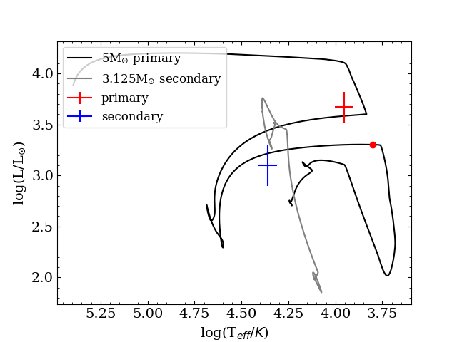
Fig. 1: The Hertzsprung-Russell diagram of the best fitting model from the paper along with the data points from the observations.

Table 1: The observational data from the paper

Like in Task 1.1 of Lab 2, the aim of this bonus task is to capture the simulations as determined from the observations of the binary system by using the src/run_binary_extras.f90. We will also inspect how adding more terms to the ${\chi }^2$ -formula will impact its value. Because the track is rather complicated, as can be seen in the figure below, we will slowly build up to finding the right combination of stopping criteria to match the models with the system. Remember to recompile the code every time you change something in the src/run_binary_extras.f90 with (./clean && ./mk) and run your new model! (./rn).

We are starting from a prepared work-directory which contains an adapted version of the published set of inlists connected to the paper mentioned earlier. You can download this here: ⬇ Download

In this lab, the focus is on working with the run_binary_extras.f90 and at the end, some visualisation in TULIPS. However, because this work directory is adapted from a scientific run, we’ll have a quick look a the setup of this directory.
When working with many different settings within MESA, it is often beneficial to split out the settings in the inlists into separate files. It might look confusing at first, so lets have a look at the inlists in this work directory. There are nine different files; inlist, inlist1, inlist2, inlist_extra, inlist_other_winds, inlist_pgstar, inlist_project, and inlist_star.

1. Open the first file, inlist, with your favourite text editor. Like in most cases, this file only refers to other inlists which contain the parameters of the run.
2. Next, open the file that inlist refers to, the inlist_project. In previous labs, the inlist_project contained all parameters. In this case, it refers to two other inlists for the settings of the primary star (inlist1) and the settings of the secondary star (inlist2). The other information in inlist_project is related to the binary physics, and it refers to the file inlist_extra.
3. The file inlist_extra contains basic settings for the binary run; the masses of the two stars and the initial period. Because these are the parameters changed in a grid-search as performed in the paper, it is easier to have them in a separate file.
4. inlist1 and inlist2 are as good as identical. The only difference between the two files is that different models are loaded and a few timestep controls. Both these inlists refer to inlist_star for star_job and control-settings and to inlist_pgstar.
5. inlist_star contains all the settings that are the same for the primary and the secondary, rather than putting them all in inlist1 and inlist2.
6. inlist_pgstar is not often used for science runs, and therefore often a separate file, so its contents are easily ignored.
7. The last inlist, inlist_other_wind, is called via the run_star_extras.f90, and contains the values used for the alternative wind-scheme that is used for this model.

Extra Bonus Task 1

In this task, the aim is to capture the point where the simulation agrees with the observational data with only one stopping criterion, the effective temperature. Because the Roche-lobe overflow phase is computationally heavy for this particular system, the run will start shortly after the mass-transfer phase, which is indicated by the red dot in Figure 1 on the track of the primary star. The saved model files are available in ‘Load’.
To make sure the models do not run too long, there is a maximum amount of models implemented in the inlist_star. To see if all runs well, compile (./clean && ./mk) and run your new model (./rn)! This is only to check if we set all the controls correctly, so kill the run after a few timesteps using Ctrl+C.
To find the stopping point, use the following parameter in the extras_binary_finish_step hook in run_binary_extras.f90:
b% s1% Teff ! Effective temperature of the primary star of the binary system in Kelvin

Then, to compare with the observational data, add a write statement to your stopping criterion to print the effective temperature and the luminosity of the stopping point.

if ((b% s1% Teff) .gt. 9000) then
   extras_binary_finish_step = terminate
   write(*,*) "terminating at requested effective temperature and luminosity:", b% s1% Teff, log10(b% s1% photosphere_L)
   return
end if

Question Do the written-out effective temperature and the luminosity match with the data in Table 1?

Extra Bonus Task 2

In Extra Bonus Task 1, we have determined that working with just the effective temperature will not lead to a match between the simulation and the observations, as the luminosity is too low compared to the observations. In this next task, we will combine the luminosity and the effective temperature of the primary star to match the observations.
Use the following additional parameter in the extras_binary_finish_step hook in run_binary_extras.f90:

b% s1% photosphere_L ! The luminosity of the primary star of the binary system in solar luminosities

if (((b% s1% Teff) .lt. 9000) .and. (log10(b% s1% photosphere_L) .gt. 3.57))   then
    extras_binary_finish_step = terminate
    write(*,*) "terminating at requested effective temperature and luminosity:", b% s1% Teff, log10(b% s1% photosphere_L)
    return
end if  

Extra Bonus Task 3

Because we are working with a binary system, it is not only important to match the primary star, but also the secondary component. However, matching two stars simultaneously is not a trivial task, and rather than fitting by eye like we are doing here, it is done with statistical methods, as was demonstrated in bonus part of Task 1.1 of Lab 2. Here, instead of monitoring ${\chi }^2$ for each timestep, only the final value at the end of the simulation will be determined. Instead of setting the calculation in extras_binary_finish_step, it will be set at the final part of the run, in extras_binary_after_evolve. To gain insight in how the different parameters of the binary system affect the ${\chi }^2$ -value, we will consider three variations;

• Only the effective temperature and luminosity of the primary
• The effective temperature and luminosity of both components
• The effective temperature and luminosity of both components as well as the period of the binary system

The values needed are given in Table 1. You can reuse the formula from Task 1.1 of the main lab.

Use the following additional parameter in the extras_binary_after_evolve hook in run_binary_extras.f90:
b% s2% Teff ! Effective temperature of the primary star of the binary system in Kelvin
b% s2% photosphere_L ! The luminosity of the primary star of the binary system in solar luminosities
b% Period ! Period of the binary system in seconds

Tip

Just as a reminder, here is the formula:

$${\chi }^2=\sum _{i=1}^n{\left(\frac{O_i-E_i}{{\sigma }_i}\right)}^2,$$

where $O_i$ is the observed value, $E_i$ is the theoretical value (in our case returned by MESA), and ${\sigma }_i$ is the observed error.

Important

The units of the MESA output and those of the observations are not the same; make sure you have the same units in the calculation.

Question What values do you get for the fit? What parameters do you think are most important to get correct?

The best-fit model presented in Gilkis & Shenar 2022 does not match the exact observational values, as can be seen in the Hertzsprung-Russell diagram below. This is also what the ${\chi }^2$ values are telling us. Especially the period of the system modelled here is off by quite a bit. However, the model presented in the paper is undergoing the second mass-transfer phase, which changes the period.

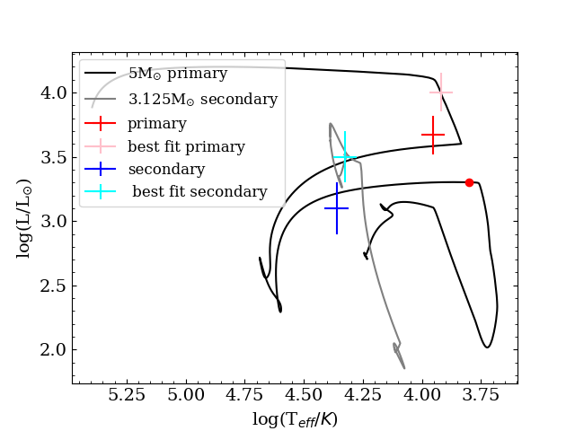
Fig. 2: The Hertzsprung-Russell diagram of the best fitting model from the paper, along with the data points from the observations and the location of the best fits.

Extra Bonus Task 4: Visualizing the stars with TULIPS

As for Lab 1, we can look at the outcome of the binary evolution in more detail by visualizing our simulations with TULIPS, a Python package for stellar evolution visualization. We will create movies of the changes in the properties of the donor and the accretor of the binary system of this lab with pre-computed input. For the visualisation, you will be using a full evolution of the system described in this Bonus Task, including the mass-transfer phases. The files necessary for this task will be downloaded through this Google Collab notebook (local copy) .
There are conceptual questions in the TULIPS Notebook. The solutions can be found here (local copy) .

Acknowledgement

The MESA input files were built upon the following resource:
Gilkis & Shenar 2022