X-ray binaries - exploring Cyg X-1

Cygnus X-1 is a well-known high-mass X-ray binary located at a distance of about 2.2 kpc, consisting of a black hole and an O-type supergiant companion. It was the first strong black hole candidate ever identified and remains one of the most extensively studied X-ray sources, exhibiting persistent emission powered by accretion from the stellar wind of the massive donor star. Recent observations by Ramachandran et al. (2025) have updated its parameters:

Orbital parameters

• $M_{\mathrm{donor}}=29_{-3}^{+6}{\mathrm{M}}_{\odot }$
• $M_{\mathrm{BH}}=17.5_{-1}^{+2}{\mathrm{M}}_{\odot }$
• $P_{\mathrm{orb}}=5.559\mathrm{d}$
• $\log \dot{M}=-6.5\pm 0.2{\mathrm{M}}_{\odot }\mathrm{y}{\mathrm{r}}^{-1}$

Physical parameters of the donor

• $T_{\mathrm{eff}}=28500\pm 1000\mathrm{K}$
• $\log L/{\mathrm{L}}_{\odot }=5.5\pm 0.1$
• $\log g=3.2\pm 0.1$
• $R=22.3_{-2.5}^{+1.5}{\mathrm{R}}_{\odot }$

The following exercises will focus on reconstructing the evolutionary history of Cygnus X-1. The goal is to identify a binary model that reproduces the observed parameters of the system.

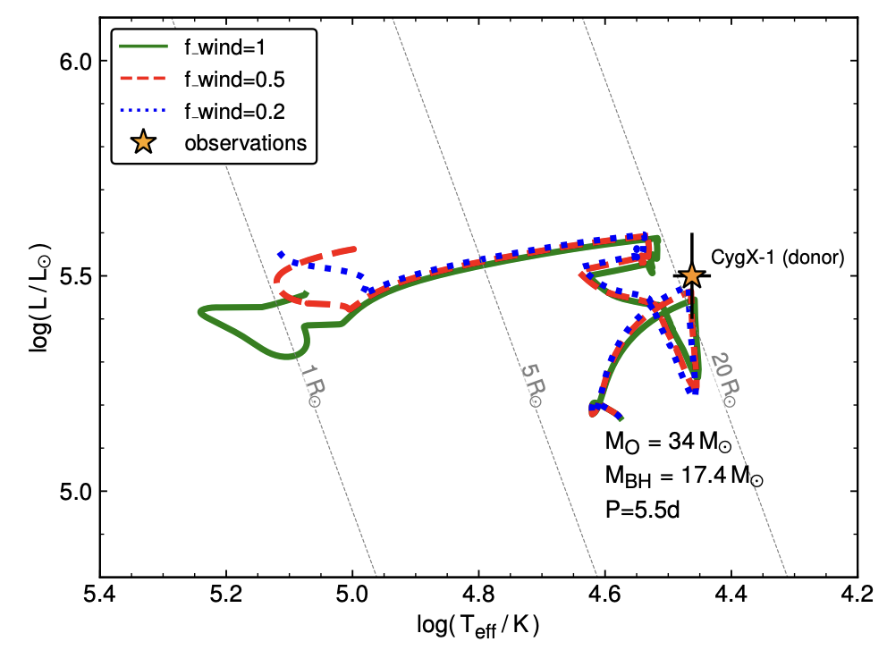
Fig. 1: The HR diagram illustrating the potential evolution of the Cyg X-1 donor star as a product of a $17.4{\mathrm{M}}_{\odot }$ black hole (point mass) and a $34{\mathrm{M}}_{\odot }$ O-type star on the $5.5$ days orbit overlaid on the observed position of the Cyg X-1 donor. The plot displays three models with different mass-loss scaling factors of $1,0.5$ , and $0.2$ to demonstrate the effect of wind mass loss on evolution (taken from Ramachandran et al., (2025))

Task 1. Simulating the Evolution of Cygnus X-1

To simulate the evolution of Cygnus X-1, we would ideally start off by creating a fresh copy of the work/ directory (cp -r $MESA_DIR/binary/work .) and modifying the inlist files to capture all relevant physical effects leading the initial system to the current form. However, to save time, we will use an already prepared MESA work directory that can be downloaded from here: ⬇ Download

Following Ramachandran et al. (2025), lets start off with setting the initial masses of the components, $M_1=34{\mathrm{M}}_{\odot },{\mathrm{M}}_2=17.4{\mathrm{M}}_{\odot }$ and orbital period $P=5.5\mathrm{d}$ in the inlist_project file, designed to contain all information about the system-related quantities. To find the controls used by MESA, look into the MESA docs, under the specifications for starting model section.

   ! Initial parameters of the system 
   m1 = 34.0d0  ! donor mass in Msun
   m2 = 17.4d0  ! companion mass in Msun
   initial_period_in_days = 5.5d0  ! initial orbital period

As the secondary component is a black hole, we assume it to be a point mass and focus only on the detailed evolution of the donor. This can be done by setting evolve_both_stars = .false. in binary_job section. Additionally, we need to set a few additional controls on the system:

• the Kolb mass transfer scheme,

   mdot_scheme = "Kolb"  

• do the wind mass accretion from the donor to the BH

   do_wind_mass_transfer_1 = .true.  

• assume conservation of the total angular momentum of the system, including loss of angular momentum via mass loss and via gravitational wave radiation

   do_jdot_ml = .true.  ! mass loss 
   do_jdot_gr = .true.  ! gravitational wave radiation
   do_jdot_ls = .true.  ! assume LS coupling due to tides

• involve the effects of tides when following the evolution of stellar rotation

     ! rotation
     new_rotation_flag = .true.
     change_rotation_flag = .true.
     change_initial_rotation_flag = .true.

To see if all runs well, compile (./clean && ./mk) and run your new model! (./rn). This is only to check if we set all the controls correctly, so kill the run after a few timesteps using Ctrl C.

Task 1.1. Finding the model that fits the observations

Based on the parameters obtained by Ramachandran et al., (2025) (see the introductory part of this lab), we can try and find the model that fits within the measured stellar parameters, like $T_{\mathrm{eff}}$ , $\log L$ and $\log g$ , and terminate the computations after doing so.

To force MESA to stop after finding a fitting model to the observations, we need to modify the run_binary_extras.f90 file. You can find it in the src/ inthe working directory. We have already prepared the file, so all you need to do is to capture the MESA quantities and to compare them with observed parameters. One of the ways is to use the observed uncertainties and to compare them with the MESA parameters:

    if ( abs(Teff_MESA - Teff_obs) < dTeff_obs) then
        ...
    end if

As we want to capture not only $T_{\mathrm{eff}}$ but also other stellar quantities, we need to expand the above example a bit.

Go ahead and add a stopping criterion extras_binary_finish_step = terminate in the extras_binary_finish_step function once a model reaches all of the desired surface properties ($T_{\mathrm{eff}}$ , $\log L$ , and $\log g$ ). Focus only on the TASK 1.1 part in run_binary_extras.f90 this time.

   ! Global parameters of Cyg X-1 
   real(dp), parameter ::  Teff_obs = 28500.0d0,  logL_obs = 5.5d0,  logg_obs = 3.2d0
   real(dp), parameter :: dTeff_obs =  1000.0d0, dlogL_obs = 0.1d0, dlogg_obs = 0.1d0

    integer function extras_binary_finish_step(binary_id)
        ...

         ! TASK 1.1
         ! Spectroscopic observations:
         !     Teff  = 28500 +/- 1000 K
         !     log_L = 5.5 +/- 0.1 Lsun
         !     log_g = 3.2 +/- 0.1
         !
         ! Apply a terminating condition, after we find a model fitting within the observed parameters
         if ( abs(b% s1% Teff - Teff_obs) < dTeff_obs .and. &
              abs(log10(b% s1% photosphere_L) - logL_obs) < dlogL_obs .and. &
              abs(b% s1% photosphere_logg - logg_obs) < dlogg_obs) then

              write(*,*) "Found a model maching the observations. Terminating"
              extras_binary_finish_step = terminate
        
        end if

    end function extras_binary_finish_step

    integer function extras_binary_start_step(binary_id,ierr)
        ...
        ! part of the bonus excercise
        !
        ! store all spectral parameters, like Teff, logL or logg 
        ! from the previous step
        Teff_old  = b% s1% Teff
        logg_old  = b% s1% photosphere_logg
        logL_old  = log10(b% s1% photosphere_L)

        ! Calculate the chi2 statistics on the previous model

        chi2_value_old = chi2(Teff_old, logL_old, logg_old, &
                            Teff_obs, logL_obs, logg_obs, &
                            dTeff_obs, dlogL_obs, dlogg_obs)

        write(*,*) 'Chi2 from the previous step:',chi2_value_old
    end function  extras_binary_start_step

    ...

    integer function extras_binary_finish_step(binary_id)
        ...
        ! part of the bonus excercise
        ! Calculate the chi2 statistics on the current model
        !
        chi2_value = chi2(b% s1% Teff, log10(b% s1% photosphere_L), b% s1% photosphere_logg, &
            Teff_obs, logL_obs, logg_obs, &
            dTeff_obs, dlogL_obs, dlogg_obs)

        write(*,*) 'Chi2 from the current step:', chi2_value
        

        ! TASK 1.1
        ! Spectroscopic observations:
        !     Teff  = 28500 +/- 1000 K
        !     log_L = 5.5 +/- 0.1 Lsun
        !     log_g = 3.2 +/- 0.1
        !
        ! Apply a terminating condition, after we find a model fitting within the observed parameters
        if ( abs(b% s1% Teff - Teff_obs) < dTeff_obs .and. &
            abs(log10(b% s1% photosphere_L) - logL_obs) < dlogL_obs .and. &
            abs(b% s1% photosphere_logg - logg_obs) < dlogg_obs .and. &
            chi2_value > chi2_value_old) then

            ...
            
            extras_binary_finish_step = terminate
        end if

    end function extras_binary_finish_step

    ...

    ! Part of the bonus excercise
    ! Create a function calculating chi2 to be called from any place in run_binary_extras 
    !
    real(dp) function chi2(Teff_mod, logL_mod, logg_mod, &
                            Teff_obs, logL_obs, logg_obs, &
                            Teff_err, logL_err, logg_err)
        real(dp), intent(in) :: Teff_mod, logL_mod, logg_mod
        real(dp), intent(in) :: Teff_obs, logL_obs, logg_obs
        real(dp), intent(in) :: Teff_err, logL_err, logg_err

        chi2 = 0.0d0
        chi2 = chi2 + ((Teff_mod - Teff_obs) / Teff_err)**2
        chi2 = chi2 + ((logL_mod - logL_obs) / logL_err)**2
        chi2 = chi2 + ((logg_mod - logg_obs) / logg_err)**2
    end function chi2

Task 1.2. Gravitational wave radiation and merger time

Fig. 2: An artist’s impression of gravitational waves in an inspiralling binary system (Credit: Caltech-JPL. R. Hurt).

Once we are all set to run our model, we can add one extra tweak to our computations. As we already assumed and implemented the loss of angular momentum via gravitational waves radiation in our model (the do_jdot_gr control in the inlist_project file), we can compute the approximate time our binary will take to merge.

For two point masses $m_1$ and $m_2$ on a circular orbit with separation $a$ , the GW inspiral time (Peters 1964) is given by

Alternatively, using orbital period $P$ instead of orbital separation:

where $M_{\mathrm{chirp}}$ is the chirp mass:

We need to do this once MESA has updated all the system parameters, thus in the extras_binary_finish_step function. We have two choices: we can force MESA to compute the merge time on a fly at every step, to be able to see how the merge time depends on the orbital period and the distribution of masses between the components, or we can implement this chunk of code inside the if statement of the previously implemented stopping criterion. As we are primarily interested in knowing the merge time at the current phase of the evolution, we can choose the second option.

      ! returns either keep_going or terminate.
      ! Note: cannot request retry; extras_check_model can do that.
      integer function extras_binary_finish_step(binary_id)
         type (binary_info), pointer :: b
         integer, intent(in) :: binary_id
         integer :: ierr

         ! Initialise new variables
         ! GRAVITATIONAL WAVES EMISSION PART 
         ! real(dp) :: mchirp, t_merge, t_merge_gyr

         call binary_ptr(binary_id, b, ierr)
         if (ierr /= 0) then ! failure in  binary_ptr
            return
         end if  
         extras_binary_finish_step = keep_going

      
         ! TASK 1.1
         ! Spectroscopic observations:
         !    Teff  = 28500 +/- 1000 K
         !    log_L = 5.5 +/- 0.1 Lsun
         !    log_g = 3.2 +/- 0.1
         !
         ! Apply a terminating condition, after we find a model fitting within the observed parameters
         ! if(...) then

             ! GRAVITATIONAL WAVES EMISSION PART 
             ! Now that we have found the quasi-best fitting model, let's compute the merger time due to GW 
             ! emission, based on Peters 1964
             !     From MESA lib: b% m(1) and b% m(2) are in grams, b% period is in seconds,
             !     const_def gives Msun, clight and standard_cgrav in cgs

         ! end if

      end function extras_binary_finish_step

    ! Initialise new variables
    ! GRAVITATIONAL WAVES EMISSION PART 
    real(dp) :: mchirp, t_merge, t_merge_gyr

    ...

    ! Chirp mass
    mchirp = ((b% m(1) * b% m(2))**(3.0d0 / 5.0d0)) / ((b% m(1) + b% m(2))**(1.0d0 / 5.0d0))

    ! t_merge in seconds
    t_merge = (5.0d0 / 256.0d0) * (clight**5 / standard_cgrav**(5.0d0 / 3.0d0)) * &
                ((b% period / (2.0d0 * pi))**(8.0d0 / 3.0d0)) * mchirp**(-5.0d0 / 3.0d0)

    ! seconds to Gyr
    t_merge_gyr = t_merge / (3600.0d0 * 24.0d0 * 365.25d0 * 1.0d9)

    write(*,*) 'Merger time [Gyr]  = ', t_merge_gyr

To apply all the changes you have made in your run_binary_extras.f90, you need to compile (./clean && ./mk) and run your model (./rn)!

Task 2. The efficiency of mass transfer and its impact on the evolution of Cyg X-1

Mass transfer in close binary systems is a highly complex, multidimensional process shaped by hydrodynamic interactions, angular momentum exchange, and geometry-dependent flow patterns. Rather than a smooth and complete handover of mass from one star to the other, the gas is channeled through the inner Lagrangian point, forming a stream that enters the Roche lobe of the companion. Depending on the relative size and position of the stars, this stream may directly impact the accretor or settle into an accretion disk before any material is finally incorporated. A significant portion of the transferred matter might never reach the companion at all, being expelled from the system via outflows, disk winds, or loss through the outer Lagrangian points.

Capturing the full physics of this process requires 3D hydrodynamical simulations, which remain computationally expensive and inaccessible for 1D routine stellar evolution modeling. In the context of 1D codes like MESA, we therefore adopt simplified prescriptions that approximate the outcome of these processes through parameterized treatments.

A central parameter in such models is the accretion efficiency, which describes the fraction of the donor’s mass loss that is successfully accreted by the companion. MESA implements this through a set of &binary_controls parameters:

• mass_transfer_alpha - fraction of mass lost from the vicinity of donor as fast wind ! (e.g., isotropic re-emission)
• mass_transfer_beta - fraction of mass lost from the vicinity of accretor as fast wind
• mass_transfer_delta - fraction of mass lost from circumbinary coplanar toroid
• mass_transfer_gamma - radius of the circumbinary coplanar toroid is ! “gamma**2 * orbital_separation”

The effective accretion efficiency is given by:

In this minilab, we will investigate how the choice of these parameters — particularly beta, which reflects wind loss near the black hole — influences the binary’s orbital and stellar evolution. We will adopt the default values of mass_transfer_alpha = 0d0, mass_transfer_delta = 0d0, and mass_transfer_gamma = 0d0 throughout, and explore a range of values for mass_transfer_beta to assess the impact of inefficient accretion in systems like Cygnus X-1. This will allow us to test how different mass loss scenarios shape the long-term configuration of the system.

Task 2.1. Varying the Mass Transfer Efficiency

To explore the effect of mass transfer efficiency on the future evolution of Cyg X-1, we will vary the efficiency of mass transfer by changing the mass_transfer_beta parameter while keeping the initial primary masses and orbital period fixed, as we did before. As each run may take a while, we will crowd-source this!

The participants should split into groups that will be assigned different values of mass_transfer_beta and limit_retention_by_mdot_edd, which is a control for the Eddington limited mass-accretion rate. To do so, please write your name in the following Google Spreadsheet (local copy; navigate to Lab2 Mass Transfer Efficiency tab in the lower-left corner if needed) to select a $\beta$ value, from 0.0, 0.1, 0.2, 0.3, 0.4, 0.5, 0.6, 0.7, 0.8, 0.9, corresponding to accretion efficiencies from 100% up to 10%, respectively. These values come either without the Eddington limit (by default) or with Eddington Eddington-limited mass-accretion rate. If you choose the latter, remember to include limit_retention_by_mdot_edd = .true. in your binary_controls section!

As the model fitting within Cyg X-1 determined parameters is right on the onset of mass transfer, let us comment out the previously applied stopping criterion from the run_binary_extras.f90 to let the system evolve a bit further. This time, let us choose the stopping criterion based on the minimum mass of the donor set to $23{\mathrm{M}}_{\odot }$ . As MESA already has a command telling it to finish a run after such a condition is met, we do not need it to be implemented inside the run_binary_extras.f90. Instead, as the limit of mass applies only to one of the components, we need to include this condition in the inlist1 file. Explore stopping conditions in the MESA docs to find the right command.

   &controls
      ...
      ! stop when mass drops below this limit
      star_mass_min_limit = 23.0d0

To make the runs a bit faster, reduce the resolution to

   &controls
   ...
      ! resolution
      mesh_delta_coeff = 2.0d0
      time_delta_coeff = 2.0d0

The last step is to compare the merge time with the one we got in the previous step. Modify slightly the run_binary_extras file, as we no longer need to calculate the merge time only for the specific model - let it be calculated for every model to see whether this value changes. Add the resulting merge time of the last computed model, when the donor reaches the minimum mass which terminates the run, to the Google Spreadsheet in the column next to your name under the selected case.

Next, compile (./clean && ./mk) and run the models (./rn) with a fixed set of initial parameters (donor and black hole masses, and orbital period), while exploring different values of mass_transfer_beta. This isolates the role of accretion efficiency in shaping the orbital evolution, mass growth, and observable properties of the system.