Minilab 3: Meridional Circulation
Introduction
So far in our exploration of rotating stellar models, we have seen how instabilities can be modeled in MESA to approximate particular behavior present in 2D-ESTER models. We have also gone further to calculate the Eddington-Sweet circulation velocity in the 1D case and seen some differences against analogous 2D references.
So what does this mean? Of course a 1D model and a 2D model are going to be different, right?
The good news is that we are not consigned to spend hours on HPC clusters for every test case. Instead, given a selective set of more expensive 2D models, we can tune our MESA models. Luckily, we have various levers we can turn to accomplish this. If we can establish an idea of what the velocity field inside the star should be, then we can implement it into MESA with hooks in run_star_extras.f90. In this lab, we will be doing just that. Beginning from a scaffolded starting point, you will implement a custom torque and angular momentum mixing routine in MESA, outputting data that can be compared against the tracks in Mombarg et al., 20231 and Mombarg et al., 20242. By tuning the torque, you can mimic the effect of meridional circulation on the behavior and evolution of the star, as given by these 2D ESTER models.
For a discussion on meridional circulation, click the hint below. This information was all covered in more detail during the lecture, so students are encouraged to only visit this discussion as needed, or while waiting for model runs to complete.
An Aside on Meridional Circulation
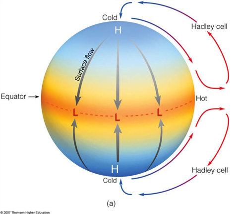
Starting from its name, meridional circulation is a convective flow that operates along the meridian (North-South). These flows are not unique to stars and are a fundamental method that energy is redistributed across rotating fluid bodies. To trigger these flows, there need to be two differentials, one along the radius, r, and one along azimuthal angle, phi, (in polar coordinates). As an example, on Earth, Hadley cells are a form of meridional circulation that is driven by thermal gradients along r (altitude) and pressure gradients along phi (latitude). As a result, heat is exchanged between the equator and higher latitudes, driving towards equilibrium. For a deeper discussion on Hadley cells, see this site from Harvard’s School of Engineering and Applied Sciences after the school. Included below is an image from that link, showing the general form of Hadley cells (specifically the possible height of the Hadley Cells during the Cretaceous)
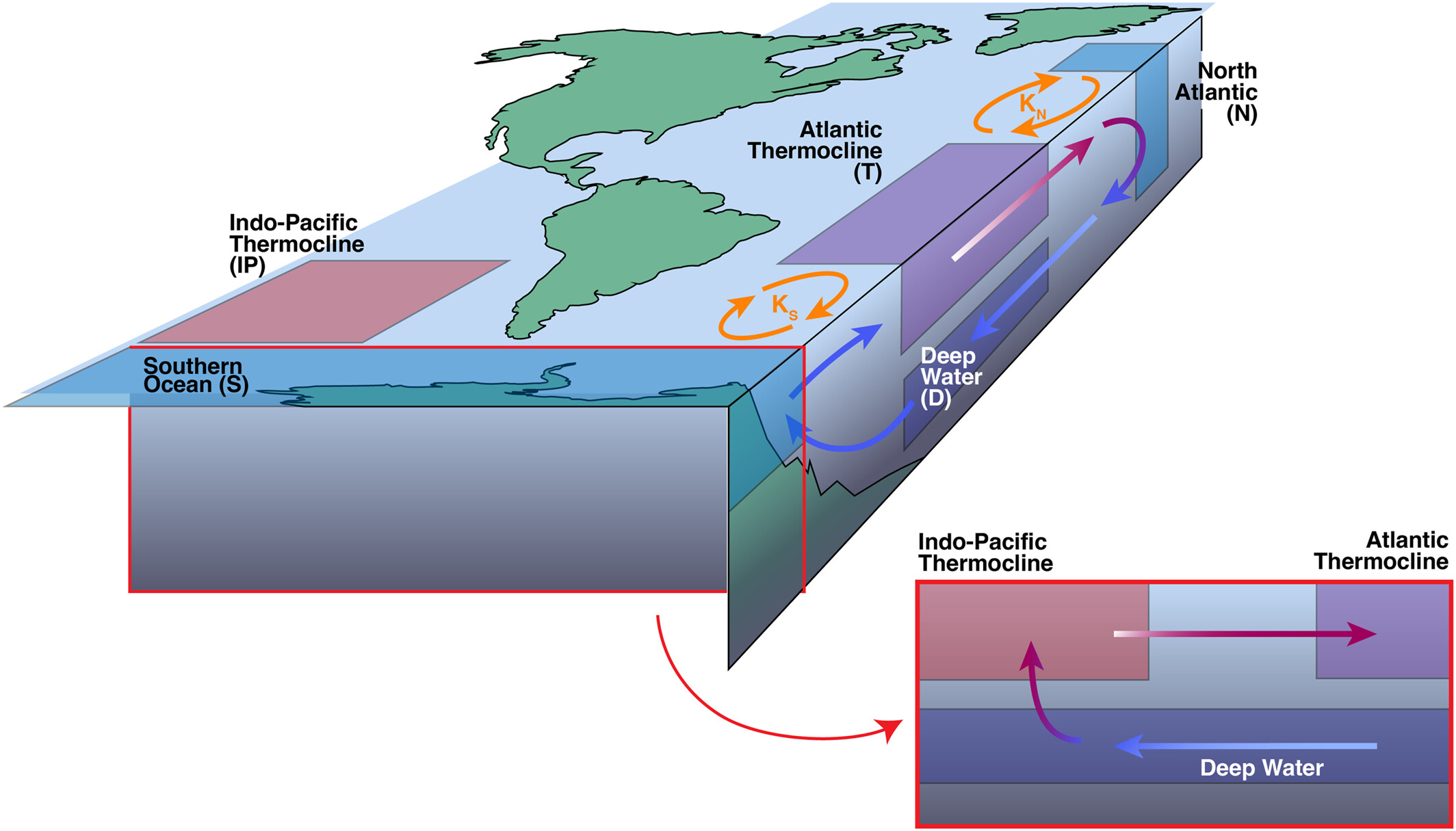
Another brief example is the Atlantic Meridional Overturning Circulation (AMOC), a key factor in global climate that transfers heat and nutrients between the equator and poles. In this case, the AMOC is driven by thermohaline gradients within the ocean (roughly, salinity along r and temperature along phi). For reference, you can check out these two links from NOAA: “What is the AMOC?” & “What is thermohaline circulation?”. Included below is a AMOC schematic from Zimmerman et al., 2025:
Of course, there is additional physics in both of these prior examples that I haven’t discussed and will leave for experts. In the realm of stars, these same complications are present. There are a number of physical forces that could be used to drive and brake these circulating cells in our model and even more papers discussing which forces are needed and which are not. At a high level, there are temperature & pressure gradients along r and differential rotation rates along phi. This drives material and energy in large cells across the star as it evolves. A 2014 discussion of meridional circulation in the Sun by Dr. Mausami Dikpati at the High Altitude Observatory can be found here.
Helpful Links
The lab setup can be found here as a mirror of the Google Drive link found below. This folder contains partial solutions (separated by task), full solutions for each test case, the starting point for the lab, pre-made ZAMS models, and a series of pre-computed runs with no meridional circulation (called no_extra_jdot).
The Google Colab script to make the bonus plots can be found here (local copy) .
Instructions
Step 0: Getting Started
| Mass | Initial |
|---|---|
| 5 | 0.60 |
| 6 | 0.60 |
| 6 | 0.75 |
| 8 | 0.60 |
| 8 | 0.75 |
| 10 | 0.60 |
| 10 | 0.75 |
| 📋 TASK 1 |
|---|
| Claim a mass and initial rotation from the table above. Coordinate with others at your table to ensure that no two people choose the same test case. |
| Download the starting point from the Google Drive to a local working directory |
This starting point should be a fairly familiar set of files. Each of these files has been -mostly- pre-prepared with the structure we will need to get going. Additionally, throughout each of these starting point files, variables that need to be changed are explicitly marked with “!!!! !!!!”. This is also true if there is some particular section that needs your input. If you have trouble finding a value, feel free to ctrl+f your way around.
| 📋 TASK 2 |
|---|
| Given the star value you selected, Download the relevant ZAMS model from the Google Drive and place it into your working directory |
The working directory should now be:
- clean
- history_columns.list
- inlist
- inlist_project
- inlist_pgstar
- mk
- profile_columns.list
- re
- rn
- ZAMS_Z02_M<mass>
- run.f90
- run_star_extras.f90
At this stage, we are now ready to dive into some inlists!
Step 1: Inlist Project
Let’s start by looking over inlist_project.
This file should be generally quite familiar from Minilabs 1 & 2. Starting from the top of the file in &star_jobs, you will need to turn on pgstar, load from the saved ZAMS model, and set the initial rotation rate. It is also recommended that you turn on the pause_before_terminate flag to ensure that you can view the pgstar plots before the script exits.
| 📋 TASK 3 |
|---|
In &star_jobs, update inlist_project to turn on pgstar, load from the saved ZAMS model, and set the initial rotation rate. |
Hint: What parameters need to be changed?
The parameters that should be updated/added are:
pgstar_flagload_saved_modelload_model_filenamenew_omega_div_omega_critpause_before_terminate<= Recommended
Next, in &controls, set the output directory for the logs, turn on the other angular momentum flag, and turn on the other torque flag. For the log directory, use a standard naming convention. It is recommended that this be something like M<mass>_Omega<initial rotation> (ie. M05_Omega0p60), but generally this is up to you. The use_other_torque and use_other_am_mixing flags are used to provide MESA with a custom subroutine that steps into the execution process and changes key behavior about how the torque and angular momentum mixing are calculated. You can explore all the available use_other_<hook> in the MESA docs here.
| 📋 TASK 4 |
|---|
In &controls, update inlist_project to set the output directory for the logs, turn on other angular momentum and turn on other torque. |
Hint: What parameters need to be changed?
The parameters that should be updated are:
log_directoryuse_other_torqueuse_other_am_mixing
We have now set the general starting conditions for the MESA model (from ZAMS). Included in these changes is a directive for MESA to look beyond its regular routines for the torque and angular momentum calculations, which we will deal with later.
Warning
Don’t forget to save your changes to the inlist!
Step 2: Inlist Pgstar
“If a MESA model runs to TAMS, and no one sees the pgstar plot, did it even happen?”
— Me, circa 2025
The provided inlist_pgstar is the same as the earlier labs for the day with two modifications. First, the bottom left plot (previously showing gravitational darkening) has been updated to plot star_age on the X-axis and log_total_angular_momentum on the Y-axis. Second, the top right plot (previously the mixing profile) has been updated to plot radius on the X-axis and log_dJ_over_J on the Y-axis. log_dJ_over_J is a new variable that we will define later that can be thought of as the contribution of our planned additional torque on the rotation profile of the star.
Note
There is no task for this step! All the relevant updates have already been made to the pgstar file.
Step 3: History/Profile Columns List
Now, we need to add some more information to the history and profile outputs of our model. Most of the values have already been added.
Surf_avg_omega, surf_avg_omega_div_omega_crit, surf_avg_v_rot, and center_omega have already been uncommented in history_columns.list. Radius, omega, r_polar, j_rot, and omega_crit have already been uncommented in profile_columns.list.
| 📋 TASK 5 |
|---|
Uncomment log_total_angular_momentum in history_columns.list. |
Uncomment omega_div_omega_crit in profile_columns.list. |
Warning
Don’t forget to save your changes to the inlists!
Step 4: Run Star Extras
As a final step before we can run the model, we need to modify src/run_star_extras.f90 to include an additional torque from meridional circulation and increase the viscosity to match the sample 2-D ESTER models.
Step 4.1: Subroutines, A New Hope
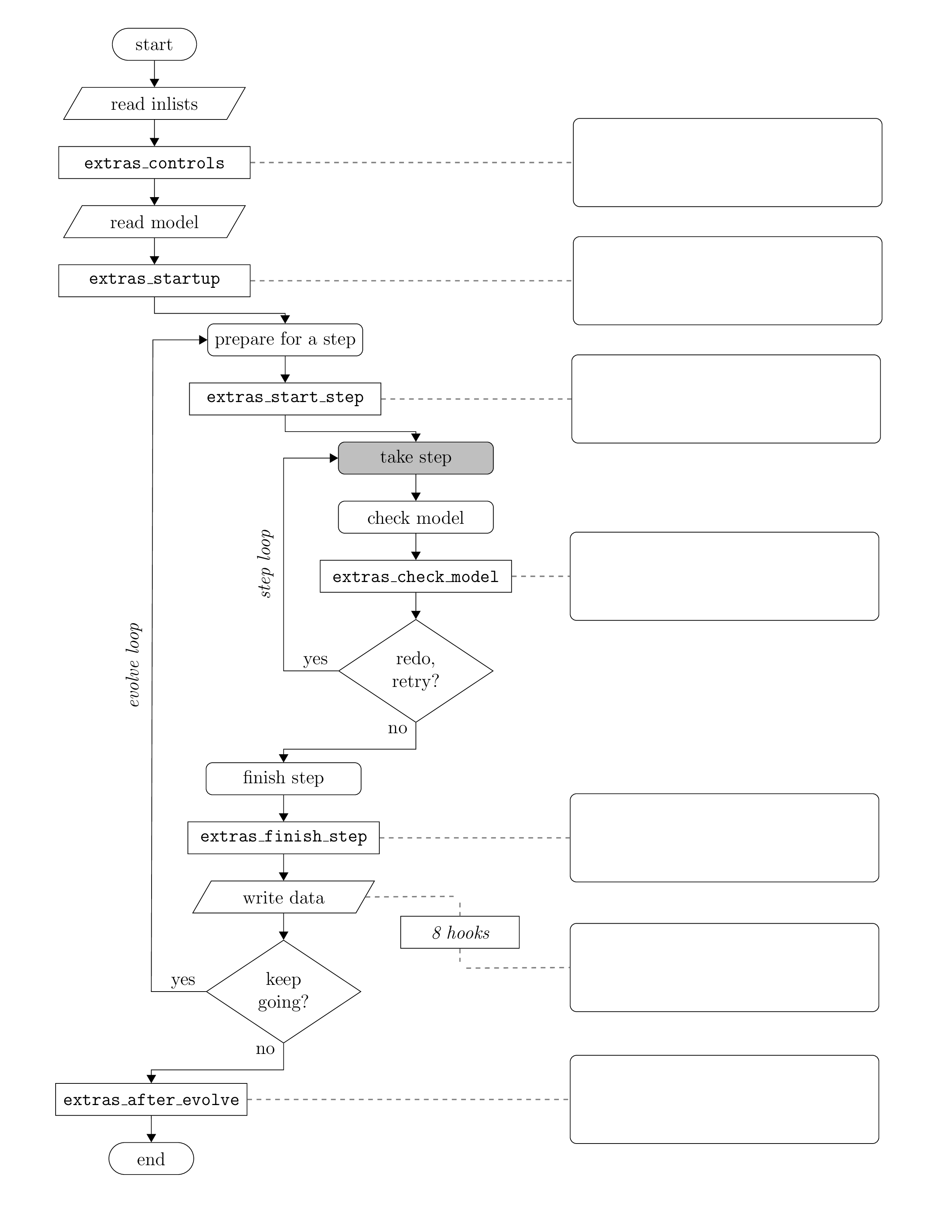
Start by looking over the run_star_extras file. Take note of the general form of the code. You will notice that this file is really a collection of labelled subroutines and functions (particularly labelled ‘integer functions’). On a high level, these are just the basic execution steps that MESA uses to solve the model. You can see when they get called in the flowchart below. This same flowchart can be found in the MESA docs here.
Super duper fun fact 🚨
The difference between a subroutine and a function in Fortran is that a function MUST return data. Subroutines, on the other hand, do not need to return anything. This short lecture by Dave Flory at Iowa State University covers some of the similarities, differences, and syntax of these structures.
These same structures exist across languages, but are not always explicitly distinguished by defining keywords. For example, in Python and Ruby, there is no real distinction between a function and a subroutine. Both structures are defined with the def keyword. Technically, a function would then include a return statement, while a subroutine would not (again, there is no real distinction here). Meanwhile, subroutines are referenced differently in Java or C by using the void keyword. This just signifies that there is not a return value.
In Step 1, we turned on two flags to use other_torque and other_am_mixing. Since we have not reached an AI Singularity (yet), MESA cannot intuit what these custom subroutines are or where they will be. Hence, we need to provide a pointer that says “This new procedure is defined by this other piece of code” in the subroutine extras_controls. The form of this pointer can be seen elsewhere in extras_controls or in the MESA docs here. Do not worry about what these custom subroutines are yet, we will cover that in the next step.
| 📋 TASK 6 |
|---|
Add in a pointer to our new custom subroutines, meridional_circulation and additional_nu. |
Hint: Pointer format
The general form of the pointer is:
s% <star procedure> => <local subroutine>Solution
s% other_torque => meridional_circulation
s% other_am_mixing => additional_nu
Step 4.2: Fortran Strikes Back
Now that MESA knows where to look, what exactly is going on in these new subroutines? In run_star_extras, scroll down to our custom other torque subroutine, meridional_circulation.
meridional_circulation is declared with the subroutine keyword, meaning we do not expact any output. Instead, this routine will grab the object containing all the star’s information, identified with the pointer s%, and modify values directly. You will also see that this subroutine takes in two values, id and ierr. id is the unique identifier that is tied to each instance of star_info, the object which holds everything about the star. ierr is an integer passed across MESA to keep tabs on the status of each operation. If this value becomes non-zero, it means that an error has occurred.
Next, we have variable declarations. In Fortran, ALL variables must be declared before they are used. This includes arrays, which have the added complication of needing to be allocated as well! The types of these variables should be explicitly provided as well. In fact, because run_star_extras.f90 contains the implicit none statement at the beginning of the file, this explicit declaration is not optional. We will need three additional integers for this subroutine: k, k0, and nz. k will be used as a counter value for the index within the model, k0 will be the index where the radiative envelope starts, and nz will hold onto the total number of zones in the model. These values will be described in more detail later.
| 📋 TASK 7 |
|---|
Declare the integers k, k0, and nz. |
Hint: What is the general form of a variable declaration?
<type> :: <variable name>Multiple variables of the same type can be declared in the same line as follows:
<type> :: <variable name0>, <variable name1>, <variable nameN>Hint: How do we declare an integer?
integer :: <variable name>Solution:
integer :: k, k0, nzNote
For a deep dive into the various types available in Fortran and more, see these notes from Ching-Kuang Shene at Michigan Technological University after the school.
Following this section, we reset the ierr integer to 0 (meaning success), grab the relevant pointer to our star object, then check if anything went wrong. This portion of the routine is functionally boilerplate. You will find the same three lines across all the routines that access an instance of the star.
The next two sections set up some important constants for subsequent calculation steps. The first, nz, is the integer number of zones in the model. This value can be accessed directly from the star pointer. The second value, k0, is the index of the zone where the radiative envelope starts. This value is not simply stored in the star pointer. Instead, we have to use a DO loop which can be thought of in the same way as a FOR loop in Python, C, or Java. This loop starts at the center and works it way to the surface, setting k0 to the first index where the mixing_type == minimum_mixing. Minimum_mixing means that the amount of diffusive mixing, D_mix, is being set to the minimum value specified in our inlist_project of 1d3. We should expect this mixing_type to switch from convective mixing to minimum_mixing only once we have entered the envelope, as we leave the convective core and enter the radiative envelope of our star. Therefore, the index where this value first switches is the base of the radiative envelope.
Important
When accessing a model array indexed by a k zone, note that k = nz represents the center of the star and k = 1 represents the surface. So, when conducting a standard incrementing loop from k = 1 to k = nz, you are sweeping from the surface into the core, NOT from the core to the surface.
Note
The criteria for what defines minimum mixing is driven by our use of set_min_D_mix and min_D_mix in inlist_project. This will not be explored further in this lab, but if you are interested in the backend operation, take a look at set_mixing_info in $MESA_DIR/star/private/mix_info.f90. Beware, the code can look a little intimidating. The relevant piece here is contained by lines 239 -> 247.
Next, we allocate and calculate three arrays: U_r, mer_comp, and dmer_comp_dr. U_r will be a simple velocity field with a constant scale factor, C, that should improve the comparison to the 2D ESTER models. Note, U_r is a by-eye linear fit to the 2D runs and NOT an actual, physical relation. The equation we will use for this field is:
mer_comp is then the meridional torque produced by that velocity field, given by:
dmer_comp_dr is then differential meridional torque per unit radius:
| 📋 TASK 8 |
|---|
Add the equation for U_r and mer_comp, assuming C = 1e-4. A reference for variable correspondence is below. |
| Variable | in MESA |
|---|---|
| s% r(i) | |
| s% rho(i) | |
| s% omega(i) |
Note
When taking the power of a value in MESA, it is recommended that you use a power function (ie. pow2(X), pow3(X), pow4(X)) as opposed to the power operator (**)
Note
When working with arrays in Fortran, basic operators and intrinsic functions are applied element-wise and return another array. So, given array A and float b, the operation A * b will produce a new array Y with the same size as A, where element Y_i = A_i * b.
Hint: How do we get R?
s% r(k) where k is the surface index, will be the total radius, R. Given that k = 1 at the surface, R = s% r(1)Solution:
U_r = (s% r) / (s% r(1)) * 0.0001 ! cm/s
mer_comp = s% rho * pow4(s% r) * (s% omega) * U_r
Note
No further changes are necessary for the meridional_circulation subroutine. The following text is a description of how this subroutine works and where copies of data are stored for Step 4.3. Feel free to skip to Task 9 to save time and use this section as reference for Tasks in Step 4.3.
We also want to store a copy of dmer_comp_dr with the star object in memory. This can be done by passing this value over to an xtraN_array, where N is an integer 1 through 6. These six of these arrays are declared within star_info to hold double precision values and are guaranteed to have a length equal to s% nz. With this array, we then call a weighted smoothing subroutine to decrease the amount of noise and increase how pretty our end plots are. We will not be exploring how the weighted smoothing subroutine works in this lab, but feel free to explore it at a later time after the school, if interested.
Fun fact
ixtraN_array) or booleansSo far, we have been doing a lot of prep work collecting variables. The next sections of the subroutine are all directed at finally applying these new torques to the model. We start at the surface and work our way down to the radiative envelope boundary k0 that we calculated previously. At each zone k we encounter, using our stored copy of dmer_comp_dr(k), we get the rate at which the specific angular momentum is changed as a result of our velocity field at t=0 and add it to whatever the value of extra_jdot was at t=-1.
Once we reach the convective core, we calculate the total torque that we applied to the envelope (saving it to a temporary value, s% xtra(1)). Then, to ensure that angular momentum is conserved across the entire star, we apply a opposing torque to zones in the core. This torque is scaled from the total torque on the envelope and in the opposite direction.
Pay attention to the places that we saved data in the star pointer, s%. Specifically, s% xtra(1) is holding onto the total torque applied to the envelope, a scalar. Meanwhile, s% xtra1_array and s% xtra2_array are storing the values of extra_jdot and dmer_comp_dr as arrays. You will need some of these values later.
You may remember that we also pointed to another subroutine, additional_nu. We will not be exploring how that subroutine works, but feel free to explore it at your own pace after the school. In practice, it is just a few DO loops to increase the viscosity and help bring the 1D model further into agreement with the 2D ESTER model.
Before we continue, we need to check that all the updates made thus far are working as expected.
| 📋 TASK 9 |
|---|
Clean, compile, and run your model. Once you see timestep outputs in the terminal, stop the run. You will likely see a few initial retry messages (retry: max residual jumped -- give up in solver). These are expected as the model tries to add the new rotation rate to the ZAMS model. |
Note
If you receive permission errors when trying to clean/make/run, you can update the file permissions with the chmod command, ie. chmod +x clean mk rn re
Step 4.3: Return of the Profile Columns (from Lab 2)
So, we have made the necessary calculations and saved off some variables into the star pointer. Now, we need to make those values presentable in the history and profile columns.
| 📋 TASK 10 |
|---|
| Add one (1) extra history column and two (2) extra profile columns. |
Hint: What values control how many extra columns there are in the history and profile outputs?
To increase the number of extra history columns, modify the variable how_many_extra_history_columns in the function how_many_extra_history_columns.
To increase the number of extra profile columns, modify the variable how_many_extra_profile_columns in the function how_many_extra_profile_columns.
Now that MESA expects some additional values, lets add the history data first.
| 📋 TASK 11 |
|---|
Add our total_torque_envelope value from Step 4.2 to a column named total_torque_envelope in the data_for_extra_history_columns subroutine. |
Hint: What is the general form of a new history column?
names(<column number>) = <your column name>
vals(<column number>) = <your value>
Hint: What is the variable containing the information we need?
s% xtra(1)Solution
names(1) = "total_torque_envelope"
vals(1) = s% xtra(1)
Now, we will need to do some calculations to get the data for the profile columns. Remember, since these are profiles, they are arrays with entries at each zone k. We will be adding two columns called extra_jdot and log_dJ_over_J. extra_jdot is the same value we encountered in meridional_circulation. log_dJ_over_J is an account of how much of the specific angular momentum was due to our additional velocity field. value can be calculated as,
where
is extra_jdot.
To put these values into columns, we need to make a DO loop across all the zones in the model, saving data in each one. An example of how to do this with a variable named beta is already given in the subroutine, data_for_extra_profile_columns.
| 📋 TASK 12 |
|---|
Add our two new profile columns, extra_jdot and log_dJ_over_J |
Hint: What is the general form of a new profile column?
names(<column number>) = <your column name>
do k = 1, nz
    vals(k, <column number>) = <your value at k>
end do
Hint: Where is extra_jdot from?
extra_jdot in the array s% xtra1_array(k).Hint: How do I write a log or absolute value in Fortran?
Use the functions below:
log10()
abs()
Hint: What other values do I need for log_dJ_over_J?
Use the functions below:
s% xtra1_array(k)
s% dt
s% j_rot(k)
Solution
names(1) = "extra_jdot"
names(2) = "log_dJ_over_J"
do k = 1, nz
    vals(k, 1) = s% xtra1_array(k)
    vals(k, 2) = log10(abs(s% xtra1_array(k) * s% dt / s% j_rot(k)))
end do
Warning
Don’t forget to save your changes to run_star_extras!
Step 5: Running the model
Let’s see MESA in action.
| 📋 TASK 13 |
|---|
| Compile and run the model. The run should continue until the model hits 510 10 timesteps. On two threads, this should take at most 8 minutes. |
Important
Do not forget to ./clean, then ./mk, then ./rn
You should see the rotation begin at your set initial value. Further along, the plot for log_dJ_over_J will display the additional torque being forced along the radius of the star. How does this value relate to the convective zone boundary? How noisy is the plot? Do you see any information about how energy is being transported?
Once the model completes, take note of the following values as printed in the pgstar plot:
center_omegasurf_avg_omegastar_age
You were also provided completed output logs & pgstar plots for each of the mass cases with extra_jdot set to a near-zero value, representing models with no meridional circulation. Importantly, in these runs extra_jdot was explicitly set to 1d-99 at each zone, k , to avoid log_dJ_over_J from becoming undefined.
| 📋 TASK 14 |
|---|
Download the directory for the no_extra_jdot case corresponding to your model from the Google Drive. |
Compare the values of center_omega, surf_avg_omega, and star_age between the cases with and without meridional circulation. |
| Compare the pgstar plots between the cases with and without meridional circulation. |
| Compare and discuss your run with others at your table. |
Pgstar Output with meridional circulation (M08, Omega 0.75)
Pgstar Output without meridional circulation (M08, Omega 0.75)
Congratulations, you have completed Lab 3! Feel free to pursue the following two bonus exercises if you have additional time.
BONUS: Recreating the results from Mombarg et al., 20242
| 📋 BONUS TASK 1 |
|---|
| Open the provided Google Colab script. |
Upload the output log directory for your run and the associated no_extra_jdot directory into the provided Google Colab notebook. Follow the steps listed there to create plots similar to those in Mombarg et al., 20242. |
| How do the plots compare? Share the plots with others at your table. Do you notice any trends? |
BONUS: Exploring other velocity field scale factors
So far we have been working through the models with an ad-hoc approximation of
with C = 1e-4.
| 📋 BONUS TASK 2 |
|---|
Explore other ranges for the constant, C, in
. |
Compare against your original run. How does modifying C change the evolution of the star? Is this expected? Why? |
Primary References
Mombarg, Joey SG, Michel Rieutord, and F. Espinosa Lara. “The first two-dimensional stellar structure and evolution models of rotating stars-Calibration to β Cephei pulsator HD 192575.” Astronomy & Astrophysics 677 (2023): L5. ↩︎
Mombarg, Joey SG, Michel Rieutord, and F. Espinosa Lara. “A two-dimensional perspective of the rotational evolution of rapidly rotating intermediate-mass stars-Implications for the formation of single Be stars.” Astronomy & Astrophysics 683 (2024): A94. ↩︎ ↩︎ ↩︎