Lab 2

Minilab 2: Modifying `run_star_extras.f90` to calculate the Eddington-Sweet circulation velocity

Led by: Philip Mocz

Goal: Compute the Eddington-Sweet circulation velocity, v_ES, for a star evolved with MESA, and save it in the profiles output. Compare it against 2D ESTER models.

MESA is quite powerful and flexible. In addition to saving all sorts of information about your star that you can request for in your inlists, MESA lets you extend its functionality by modifying the run_star_extras.f90 file. This allows you to compute and save additional quantities, such as v_ES, directly into the profiles output for further analysis. For these operations, you will need to code in Fortran and learn about MESA’s data structures and subroutines. This flexibility enables you to customize your simulations and extract specific data tailored to your research needs.

Theory

The paper Heger et al. (2000) defines the Eddington-Sweet velocity, reproduced below. For this lab, do not worry about understanding this formula! Our goal is to take it at face-value and implement its calculation in MESA.

The Eddington-Sweet velocity $v_{ES}$ is the difference between an estimate for the circulation velocity (absolute value) minus a meridional circulation correction term:

v_{ES} \equiv max (∣ v_{e} ∣ - ∣ v_{μ} ∣, 0)

From Kippenhahn (1974), the estimate of the circulation velocity is:

v_{e} \equiv \frac{\nabla _{ad}}{δ ( \nabla _{ad} - \nabla )} \frac{Ω ^{2} r ^{3} l}{( G m ) ^{2}} [\frac{2 ( ε _{n} + ε _{v} ) r ^{2}}{l} - \frac{2 r ^{2}}{m} - \frac{3}{4 π ρ r}]

In the presence of $μ$ -gradients, meridional circulation has to work against the potential and thus might be inhibited or suppressed (Mestel 1952, 1953). Formally, this can be written as a “stabilizing” circulation velocity,

v_{μ} \equiv \frac{H _{P}}{τ _{KH}^{*}} \frac{φ \nabla _{μ}}{δ ( \nabla - \nabla _{ad} )}

(Kippenhahn 1974; Pinsonneault et al. 1989), where

τ_{KH}^{*} \equiv \frac{G m ^{2}}{r ( l - m ε _{v} )}

is the local Kelvin-Helmholtz timescale, used here as an estimate for the local thermal adjustment timescale of the currents (Pinsonneault et al. 1989).

More on what all these variables are in a bit! Note: As a reference, MESA does compute the Eddington-Sweet velocity internally in the file star/private/rotation_mix_info.f90

Project work directory

📋 TASK 0
Download the `lab-2/` working directory.

We will start with a clean project work directory lab-2/, which sets up a 10 solar mass rotating star, similar to lab-1 from today which you just completed. The star setup is defined in your inlist: inlist_project and the setup for plotting with pgstar is in the file inlist_pgstar. For this lab, we will be modifying the src/run_star_extras.f90 Fortran file to add new computations into MESA.

Extending MESA

The MESA Documentation at https://docs.mesastar.org is very useful for describing how to use and modify MESA. The page Extending MESA describes, for example, how to compute and save an extra profile by modifying your run_star_extras.f90 file in your project work directory.

The run_star_extras.f90 file contains hooks to modify the output profile columns.

how_many_extra_profile_columns
data_for_extra_profile_columns

(Note: there are also hooks to add custom history columns)

The first function (how_many_extra_profile_columns) needs to be modified to tell MESA how many columns to add. In our case we are interested in adding one new column, so the function should look like:

integer function how_many_extra_profile_columns(id)
   integer, intent(in) :: id
   integer :: ierr
   type (star_info), pointer :: s
   ierr = 0
   call star_ptr(id, s, ierr)
   if (ierr /= 0) return
   how_many_extra_profile_columns = 1
end function how_many_extra_profile_columns

instead of

integer function how_many_extra_profile_columns(id)
   integer, intent(in) :: id
   integer :: ierr
   type (star_info), pointer :: s
   ierr = 0
   call star_ptr(id, s, ierr)
   if (ierr /= 0) return
   how_many_extra_profile_columns = 0
end fun

Note: the only line that has changed is that we switched the variable how_many_extra_profile_columns = 0 to how_many_extra_profile_columns = 1, to indicate that want to add a new profile to compute in the output.

📋 TASK 1
Modify the `how_many_extra_profile_columns` function `run_stars_extras.f90` file in your work directory now to look like the above.

Solution. Click on it to check your solution.

Your function should look like the following.

integer function how_many_extra_profile_columns(id)
   integer, intent(in) :: id
   integer :: ierr
   type (star_info), pointer :: s
   ierr = 0
   call star_ptr(id, s, ierr)
   if (ierr /= 0) return
   how_many_extra_profile_columns = 1
end function how_many_extra_profile_columns

The second function (data_for_extra_profile_columns) will perform the calculation. In this lab, you will fill out this function.

subroutine data_for_extra_profile_columns(id, n, nz, names, vals, ierr)
   integer, intent(in) :: id, n, nz
   character (len=maxlen_profile_column_name) :: names(n)
   real(dp) :: vals(nz,n)
   integer, intent(out) :: ierr
   type (star_info), pointer :: s
   integer :: k
   integer :: i
   ierr = 0
   call star_ptr(id, s, ierr)
   if (ierr /= 0) return

   ! TODO: IMPLEMENT EDDINTGON-SWEET VELOCITY CALCULATION HERE

   names(1) = ! TODO: NAME OF MY NEW CUSTOM PROFILE COMPUTATION
   do i = 1, nz
      vals(i,1) = ! TODO: VALUE OF MY PROFILE AT ZONE i
   end do

   end subroutine data_for_extra_profile_columns

📋 TASK 2
Implement the calculation of the Eddington-Sweet velocity inside the `data_for_extra_profile_columns` function now, using the guide below.

Again, the equation is:

v_{e} \equiv \frac{\nabla _{ad}}{δ ( \nabla _{ad} - \nabla )} \frac{Ω ^{2} r ^{3} l}{( G m ) ^{2}} [\frac{2 ( ε _{n} + ε _{v} ) r ^{2}}{l} - \frac{2 r ^{2}}{m} - \frac{3}{4 π ρ r}]

where

v_{μ} \equiv \frac{H _{P}}{τ _{KH}^{*}} \frac{φ \nabla _{μ}}{δ ( \nabla - \nabla _{ad} )}

and

τ_{KH}^{*} \equiv \frac{G m ^{2}}{r ( l - m ε _{v} )}

You will have to specify the name of the new profile column, e.g. names(1) = 'v_ES', and its values vals(i,1), where i is the i-th zone in the star. There are nz zones in total. The index 1 refers to the fact that this is the 1st extra column we are filling out.

To calculate the Eddington-Sweet velocity, we will need to know the variable names in the code that correspond to the ones in the equation. I provide a reference below:

Variable	in MESA	physical meaning
$\nabla_{ad}$	s% grada(i)	adiabatic temperature gradient
$δ$	s% chiT(i) / s% chiRho(i)	ratio of $d ln P_{eos} / d ln T$ at constant $ρ$ and $d ln P_{eos} / d ln ρ$ at constant $T$
$r$	s% r(i)	radial coordinate
$l$	s% L(i)	luminosity profile
$m$	s% m(i)	mass profile
$ρ$	s% rho(i)	density profile
$ε_{n}$	s% eps_nuc(i)	total energy (erg/g/s) from nuclear reactions
$\nabla - \nabla_{ad}$	s% gradT_sub_grada(i)	difference between temperature gradient and adiabatic temperature gradient. (recall: $\nabla > \nabla_{ad}$ means convectively unstable)
$G$	s% cgrav(i)	gravitational constant (note: MESA let’s you modify the graviational strength, hence a zone-wise value)
$Ω$	s% omega(i)	rotation frequency
$H_{P}$	s% scale_height(i)	scale height
$B$	s% smoothed_brunt_B(i)	$\frac{φ}{δ} \nabla_{μ}$

For our purposes, we can ignore $ε_{ν}$ (neutrinos) in our calculations.

Fortran has built-in functions liks abs() and max(), which may be useful. We also have access to the variable pi through the constants (const) module.

In Fortran, if you want to create new variables to store intermediate calculations, we need to declare them at the top of your function.

For example, to declare a new decimal number called, let’s say delta, do:

real(dp) :: delta

and to declare a new integer, e.g. m, do:

integer :: m

At this point you can go ahead and implement the formula yourself, but below are a few more details fleshed-out if you are feeling stuck.

Let’s start by computing $δ$ , i.e., the code variable delta. First, declare the variable as above at the indicated line in the run_star_extras. Then, in the do-loop, define delta as the ratio of s% chiT(i) and s% chiRho(i).

do i = 2, nz
      delta = s% chiT(i) / s% chiRho(i)
      ! rest of your solution here ...
end do

Next, we define a real(dp) :: denom the same as delta, which will be everything in the dominator in the factor before the bracket term on the right-hand side of the expression of v_e. In the do-loop, define denom. Since the star_info contains $\nabla - \nabla_{ad}$ and not $\nabla_{ad} - \nabla$ we have to take its negative value. To raise a quantity to an integer power, say square it, you can use pow2(s% cgrav(i) * s% m(i)))

You should now have something like this

do i = 2, nz
      delta = s% chiT(i) / s% chiRho(i)
      denom = (-s% gradT_sub_grada(i) * delta * pow2(s% cgrav(i) * s% m(i)))
      ! rest of your solution here ...
end do

Now, we compute the estimate for the circulation velocity $v_{e}$ , i.e., a new intermediate code variable I’ve called ve0 in the solution, which is $\nabla_{ad} Ω^{2} r^{3} l$ times the product of the denominator and the term in brackets. The term in brackets is already pre-defined in the run_star_extras for you as bracket_term. (Do not forget to declare ve0!) So ve0 = ... * bracket_term/denom.

Now we are almost there. Lastly, set the value of the extra profile column equal to $v_{ES} \equiv max (∣ v_{e} ∣ - ∣ v_{μ} ∣, 0)$

The velocity $v_{μ}$ is also already defined for you in the solution as ve_mu. In the do-loop add, update the line vals(i,1) = …` with the correct final expression for the Eddington-Sweet velocity we want the function to return.

Hint 1.

Naming the new profile column should look like this, inside the data_for_extra_profile_columns() function:

names(1) = 'v_ES'

Hint 2.

A few calculated terms may look like the following:

delta = s% chiT(i) / s% chiRho(i)
! Heger+2000 Eqn. (35)
bracket_term = 2.0d0 * s% r(i) * s% r(i) * (s% eps_nuc(i)/(s% L(i)) - 1.0d0/(s% m(i))) - 3.0d0 / (pi4 * s% rho(i) * (s% r(i)))
denom = (-s% gradT_sub_grada(i) * delta * pow2(s% cgrav(i) * s% m(i)))
ve0 = s% grada(i) * s% omega(i) * s% omega(i) * s% r(i) * s% r(i) * s% r(i) *s% L(i) * bracket_term/denom

(Don’t forget to declare new parameter names, e.g. real(dp) :: delta, bracket_term, denom, ve0, at the top of the function in Fortran!)

Solution. Click on it to check your solution.

Your function should look like the following.

subroutine data_for_extra_profile_columns(id, n, nz, names, vals, ierr)
   integer, intent(in) :: id, n, nz
   character (len=maxlen_profile_column_name) :: names(n)
   real(dp) :: vals(nz,n)
   integer, intent(out) :: ierr
   type (star_info), pointer :: s
   integer :: k
   integer :: i
   real(dp) :: alfa, delta, bracket_term, denom, ve0, t_kh, ve_mu
   ierr = 0
   call star_ptr(id, s, ierr)
   if (ierr /= 0) return

   ! note: do NOT add the extra names to profile_columns.list
   ! the profile_columns.list is only for the built-in profile column options.
   ! it must not include the new column names you are adding here.

   ! here is an example for adding a profile column
   ! Eddington-Sweet circulation velocity
   if (n /= 1) stop 'data_for_extra_profile_columns'
   names(1) = 'v_ES'
   vals(1,1) = 0.0d0

   ! SOLUTION
   do i = 2, nz
      delta = s% chiT(i) / s% chiRho(i)
      ! Heger+2000 Eqn. (35)
      bracket_term = 2.0d0 * s% r(i) * s% r(i) * (s% eps_nuc(i)/(s% L(i)) - 1.0d0/(s% m(i))) - 3.0d0 / (pi4 * s% rho(i) * (s% r(i)))
      denom = (-s% gradT_sub_grada(i) * delta * pow2(s% cgrav(i) * s% m(i)))
      ve0 = s% grada(i) * s% omega(i) * s% omega(i) * s% r(i) * s% r(i) * s% r(i) *s% L(i) * bracket_term/denom
      t_kh = s% cgrav(i) * s% m(i) * s% m(i) / (s% r(i) * (s% L(i)))
      ve_mu = (s% scale_height(i)/t_kh) * (s% am_gradmu_factor * s% smoothed_brunt_B(i)) / (s% gradT_sub_grada(i))
      vals(i,1) = max(0._dp, abs(ve0) - abs(ve_mu))
   end do
   
end subroutine data_for_extra_profile_columns

Searching the codebase for variables

You can find out what each variable exactly does in MESA by searching around in the code with the grep command-line tool. All the variables available can be found in the star_data/public/*.inc include files, and their default values found in star/defaults/controls.defaults. To see where they appear in the source code, you’ll need to search the Fortran *.f90 source code files. E.g., go to your main MESA directory,

cd $MESA_DIR

and try out the following:

grep am_gradmu_factor star/defaults/controls.defaults
grep am_gradmu_factor star_data/private/*.inc
grep am_gradmu_factor star/private/*.f90

to see all appearances and uses of am_gradmu_factor in the code.

Bonus

For numerical robustness, MESA sometimes internally smooths calculated variables across zones. For example, a smoothed variant of our variable $δ$ averaged across two zone looks like the following:

! alpha smoothing
alfa = s% dq(i-1) / (s% dq(i-1) + s% dq(i))
delta = alfa * s% chiT(i) / s% chiRho(i) + (1.0d0 - alfa) * s% chiT(i-1) / s% chiRho(i-1)

Use this smoothed calculation of $δ$ in your run_star_extras.f90 file, instead of a single zone lookup. Investigate the result of alpha-smoothing on $δ$ on your calculation of the Eddington-Sweet velocity profile.

Run your MESA simulation

📋 TASK 3
Compile and Run your simulation, using the instructions below.

Once you have implemented the Eddington-Sweet velocity, we will need to compile the code in your work directory and run it. To compile, do:

./mk

and to run, do:

./rn

The simulation will take a few minutes, and we’ve added custom code to plot the Eddington-Sweet velocity in pgstar as your simulation runs.

Note: as you implement your calculation in run_stars_extras.f90 and try to compile the code with ./mk, you may run into bugs and error messages. The TA Team can help debug them.

Compare your results against 2D ESTER models

📋 TASK 4
Plot your simulation results against 2D ESTER models, using the instructions below.

To plot your final MESA results against 2D ESTER models, we will use the Python library mesa-reader by Bill Wolf. If you have Python installed on your system, you’ll need to install mesa-reader (e.g., pip install mesa-reader), and run the plotting script provided in your work directory:

python plot.py

Otherwise you can visit the following Google Colab notebook and make the plot it in the cloud:

Google Colab MESA Day 2 Minilab 2 notebook (local copy) .

You’ll need to upload the MESA output (the files inside M10_Z0p20_fov0p015_logD3_O20/) and the ESTER mode (ester_models/M10_O60_X071Z200_evol_viscv1e7_visc_h1e7_delta010_2_0025.h5) into the /content/ folder and press Run to create the plot.

Solution. Click on it to check your solution.

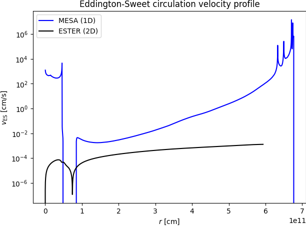Plotting the comparison between your 1D MESA model and a 2D ESTER model will look like this: landscape

As you can see, a simple 1D MESA model does not accurately capture all details of a detailed 2D rotating model, although it does capture many of its global properties as a function or rotation rate.

Lab 1 Lab 3

Minilab 2: Modifying run_star_extras.f90 to calculate the Eddington-Sweet circulation velocity

Theory

Project work directory

Extending MESA

Searching the codebase for variables

Bonus

Run your MESA simulation

Compare your results against 2D ESTER models

Minilab 2: Modifying `run_star_extras.f90` to calculate the Eddington-Sweet circulation velocity