Lab 1: 1D rotating stellar models
Introduction
In the most simple case of a non-rotating single star, the only forces acting on a mass element are pressure and gravity. The resulting spherical symmetry implies that the stellar structure equations depend only on one spatial coordinate (mass or radius) and time. However, rotation breaks the spherical symmetry consequently affecting stellar surface parameters, abundances and even its course of evolution (see e.g. Palacios 2013). To properly account for all the effects associated with rotation we need a multidimensional approach to solve the stellar structure equations. Today, we will compute 1D MESA rotating models and compare them with 2D ESTER models (Mombarg et al, 2023; 2024).
MESA includes rotational effects by applying corrections to the equilibrium stellar structure equations to account for the effect of the centrifugal force and by solving two additional equations: the mixing of chemical elements and the angular momentum (AM) transport. The latter determines the evolution of the angular velocity with time which is what we will focus on this lab 1.
The AM transport is mediated through diffusive and advective processes. In MESA, the AM transport is only included by diffusion using the following equation,
where is a shell specific moment of inertia, and is the turbulent viscosity which determines the efficiency of the AM transport. The first term on the right-hand side accounts for the diffusion transport and the second term accounts for contraction and expansion of the shells at constant mass.
In this lab 1 we will incorporate rotation in a 10 solar mass model using MESA. We will look at the effect of rotation in the global surface parameters and on the internal rotation profile by including different AM transport mechanisms.
| 📋 TASK example |
|---|
| Throughout the lab 1 you will find the specific tasks you need to execute inside boxes like this one. |
Download our template
| 📋 TASK |
|---|
| 1. Download the starting point working directory for lab 1 and the solutions for each exercise here. |
2. Unpack the zip files using unzip lab1.zip and move to the working directory cd lab1/starting_point. |
Create a 10 solar mass rotating main-sequence model
We will start by creating a rotating main-sequence model for a 10 solar mass star. To save some computation time we already computed the pre-main sequence (PMS) track beforehand and saved the model once it reached the zero-age-main-sequence (ZAMS). You will use this ZAMS model as the starting point of all your runs. The particular ZAMS model we provide matches the 2D ESTER models composition, which we will use later.
inlist_project
In this lab we only need to modify the &star_job and &controls sections of the inlist_project. You can find all the commands available in MESA for the &star_job section here and for the &controls section here.
star_job
Let’s start by modifying the &star_job section of the inlist_project. First, you need to indicate that you do not want to create a PMS model. Then, you need to load the precomputed model_ZAMS in your work directory to start the computation from that point.
| 📋 TASK |
|---|
1. Look for the three parameters you need to add to the inlist_project in the MESA &star_job documentation here in order to load the precomputed model_ZAMS. |
Hint.
starting modelSolution. Click on it to check your solution.
These are the three parameters you need to add to the &star_job portion of the inlist_project.
create_pre_main_sequence_model = .false.
load_saved_model = .true.
load_model_filename = 'model_ZAMS'
The degree of deformation from the spherical symmetry due to rotation depends on the ratio of the rotation rate and the critical rotation of the star ( ). The critical rotation is reached when the centrifugal force equals the gravitational force in the equatorial plane.
For this run, we will create a slow rotating model with = 0.2. Since our PMS model did not include rotation, you need to include additional steps for the numerical scheme to relax to the set initial rotation rate when including rotation in the ZAMS.
| 📋 TASK |
|---|
1. Add the following lines to the &star_job portion of the inlist_project to set the
= 0.2. |
new_omega_div_omega_crit = 0.2d0
set_near_zams_omega_div_omega_crit_steps = 20
controls
Next, in the &controls section add a stopping criterion when the central hydrogen abundance drops below
, i.e. at the end of the main-sequence stage.
| 📋 TASK |
|---|
1. Look for the two parameters you need to add to the &controls section in the inlist_project to determine when to stop the run. You find the MESA &controls documentation here. |
Hint.
when to stop tab and search for the key-word xa_central_lower_limit.Solution. Click on it to check your solution.
xa_central_lower_limit_species(1) = 'h1'
xa_central_lower_limit(1) = 1d-3
As we introduced in the beginning of this lab, the turbulent viscosity coefficient determines the efficiency of the transport of AM by diffusion. A very high value of induces very efficient AM transport and results in near solid body rotation rate as it is the case in convective regions.
For the purpose of this lab we will include an arbitrary viscosity coefficient that is uniform throughout the star.
| 📋 TASK |
|---|
1. Look for the two parameters you need to add to the inlist_project in the MESA &controls documentation here. The MESA parameter for the viscosity
is am_nu. |
| 2. In this case, set to a value of 1d5. |
Hint.
uniform_am_nu. Since we are adding an ad-hoc value for the viscosity (not a viscosity value derived from hydrodynamic rotational instabilities) the parameters you are looking for contain *_non_rot in the name.Solution. Click on it to check your solution.
These are the two parameters you need to add to the &controls portion of the inlist_project.
set_uniform_am_nu_non_rot = .true.
uniform_am_nu_non_rot = 1d5 !cm^2/s
Lastly, modify the output LOGS directory name to specify the physics you included in your model, for example LOGS_0.2_nuvisc_1d5. Do not forget to change the name of the LOGS directory in each run otherwise the output files will be overwritten.
| 📋 TASK |
|---|
1. Add the following lines to the &controls portion of the inlist_project to modify the LOGS directory name. |
2. Replace the <> according to the physics included in your model. |
log_directory = 'LOGS_<omega/omega_crit>_nuvisc_<am_nu_value>'history_columns.list
Now that we have included the rotation parameters in our inlist let’s add the rotation variables to the history.data file so that we can track how those parameters change along evolution. To do so, you just need to modify the file history_columns.list located in your work directory.
| 📋 TASK |
|---|
1. Uncomment (remove the ! ) the lines below from the file history_columns.list. You can do ctr+f to find the variables. |
surf_avg_omegasurf_avg_omega_div_omega_critgrav_dark_L_polargrav_dark_Teff_polargrav_dark_L_equatorialgrav_dark_Teff_equatorial
profile_columns.list
Let’s also add the rotation profile information to the profile.data files by modifying the file profile_columns.list in your work directory.
| 📋 TASK |
|---|
1. Uncomment (remove the ! ) the lines below from the file profile_columns.list. |
omegaomega_div_omega_crit
Important
Do not forget to save all the changes you made in the inlist_project, history_columns.list and profile_columns.list.
Note
We remind you that you can consult the solutions of the tasks here.
MESA run
Now that we have included the relevant physics in our inlist let’s start the computation. Do not forget to always clean the executable files, compile the code and, run the executable file generated. The run will stop automatically after it reaches the stopping criterion (this might take some minutes < 5min).
| 📋 TASK |
|---|
1. Finally let’s run MESA. To do so, run the following commands on your terminal ./clean ./mk ./rn. |
Tip
If you get permission denied when trying to ./mk or ./rn, run chmod u+x clean mk rn in the terminal.
Note
A pgplot window should appear when you start the MESA run. Spend some time looking at the pgplot to understand each individual plot.
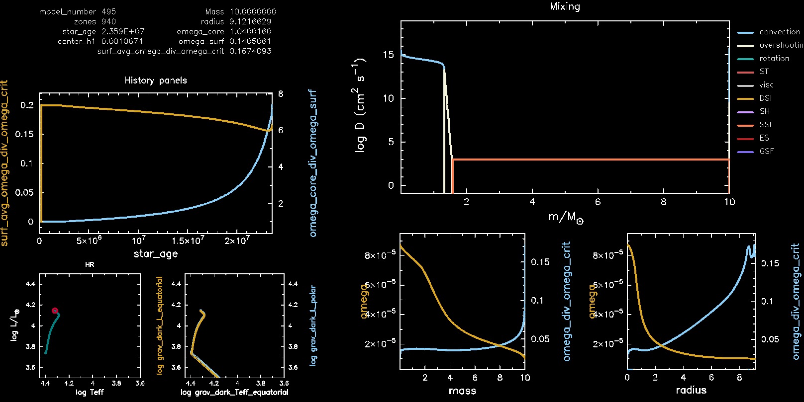
You should be looking at the following plots:
- Top left: evolution of surface rotation rate divided by the critical rotation rate (left axis) and the ratio between the near core and surface rotation rate (right axis);
- Two small panels bottom left: HR diagram as seen from different angles. The left panel shows the intrinsic variables, the right panel shows the polar and equatorial variables;
- Top right: the mixing panel (already seen on Monday);
- Two panels bottom right: the rotation rate against mass and radius.
Don’t worry if your run has finished before you grasped the content of the plots. The pgplot of the final model was saved in the /png folder under the name grid1000200.png.
| 📋 TASK |
|---|
1. Modify the name of this file in order to not be rewritten in the next runs, for e.g. grid1000200_0.2_nuvisc1d5.png. |
At the end of your run your pgstar plot should look like this.
The effect of rotation on the surface parameters
We will now look at the effect of rotation in the global surface parameters. To do so we need to increase the rotational velocity in our models.
inlist_project
Let’s modify our inlist_project to create another model with the same physics as our previous model but with faster rotation.
| 📋 TASK |
|---|
1. Make the necessary modifications to the inlist_project to set
= 0.6. |
2. Change the LOGS directory name, for e.g. 'LOGS_0.6_nuvisc_1d5'. |
Solution. Click on it to check the parameters you need to modify.
Modify the parameter in the &star_job section of the inlist_project.
new_omega_div_omega_crit = 0.6d0Modify the parameter in the &controls section of the inlist_project.
log_directory = 'LOGS_0.6_nuvisc_1d5'Important
Do not forget to save all the changes you made in the inlist_project.
MESA run
Let’s run MESA again. The run will stop automatically after it reaches the stopping criterion (this might take some minutes < 5min).
After the run has finished do not forget to modify the png file name, for e.g. grid1000495_0.6_nuvisc1d5.png.
| 📋 TASK |
|---|
1. Run MESA: ./rn |
Note
A pgplot window should appear when you start the MESA run.
| 📋 TASK |
|---|
| 1. Compare the pgplot png files of the two runs ( = 0.2 and = 0.6), more specifically compare the HR diagram panels. Can you explain why they are different? |
| 2. Discuss with your table your conclusions. |
Discuss with your table first before clicking here.
(Magneto)-hydrodynamic instabilities
In the previous task we took a very simple approach by including a constant ad-hoc viscosity in MESA models. Now, we will take a more physically motivated approach by including (magneto)-hydrodynamic instabilities in our stellar models.
In addition to the effects of rotation on the surface parameters, rotation also triggers several hydrodynamical instabilities that can transport AM and chemical elements in the radiative regions. MESA includes several (magneto)-hydrodynamical (MHD) processes in its AM transport prescription:
- dynamical shear instability (DSI),
- Solberg-Høiland instability (SH),
- secular shear instability (SSI),
- Eddington-Sweet circulation (ES),
- Goldreich-Schubert-Fricke instability (GSF),
- Spruit-Taylor dynamo (ST).
See more details on these physical processes in Heger et al. (2000).
In this exercise we will compute models with different and different rotational-instabilities.
| 📋 TASK |
|---|
| 1. Choose a and a combination of rotational-instabilities from this google spreadsheet (local copy). |
| 2. Fill the google spreadsheet with your name so that no one computes the same model. |
Tip
Choose the lower to start with since they are easier to compute. If by the end of the lab you still have time to spare you can run a different combination from the spreadsheet.
inlist_project
Let’s modify inlist_project according to what you have chosen in the google spreadsheet.
First, we need to disable the uniform viscosity in the &controls section of the inlist_project that we used in the previous exercise.
| 📋 TASK |
|---|
1. Add the following lines to the &controls portion of the inlist_project. |
set_uniform_am_nu_non_rot = .false.
uniform_am_nu_non_rot = 0d0
Next, we will include the AM transport by (magneto)-hydrodynamic processes in our run. In MESA, the viscosity coefficient is calculated as a sum of the diffusion coefficients for convection, semi-convection and the (magneto)-hydrodynamical instabilities described above.
| 📋 TASK |
|---|
1. Add the following lines to the &controls portion of the inlist_project. |
2. Set the respectives D_<INSTABILITY>_factor = 1 according to the instabilities you have chosen. |
D_DSI_factor = 0d0   ! dynamical shear instability
D_SH_factor  = 0d0   ! Solberg-Hoiland
D_SSI_factor = 0d0   ! secular shear instability
D_ES_factor  = 0d0   ! Eddington-Sweet circulation
D_GSF_factor = 0d0   ! Goldreich-Schubert-Fricke
D_ST_factor  = 0d0   ! Spruit-Tayler dynamo
Lastly, you need to modify the according to the value you chose in the Google spreadsheet. Remember that we have already done this step in the previous tasks.
| 📋 TASK |
|---|
1. Modify inlist_project to set the chosen value of
. |
2. Change the LOGS directory name, for e.g. 'LOGS_0.6_DSI'. |
Solution. Check here the parameters you have to modify.
Modify the parameter in the &star_job section of the inlist_project.
new_omega_div_omega_crit = <VALUE>Modify the parameter in the &controls section of the inlist_project.
log_directory = 'LOGS_<VALUE>_<INSTABILITY>'Important
Do not forget to save all the changes you made in the inlist_project.
MESA run
Finally let’s run MESA! The run will stop automatically after it reaches the stopping criterion (this should take some minutes < 5min). After the run has finished do not forget to modify the png file name, for e.g. grid1000495_0.6_DSI.png.
| 📋 TASK |
|---|
1. Run MESA: ./rn |
Note
A pgplot window should appear when you start the MESA run.
Look at the mixing panel (large panel on the upper right-hand side) to confirm that the instability you included in the inlist_project was activated.
See how the rotation profile evolves with time.
After your run is finished, open the history.data file in your favourite text editor and look in the last line (which corresponds to the last computed model) for the data required to fill in the google spreadsheet.
| 📋 TASK |
|---|
1. Insert the values of omega_core omega_surf and surf_avg_omega_div_omega_crit of your last model in the google spreadsheet. |
Comparison with 2D Ester models
The last task in this lab1 is to compare your MESA tracks with 2D Ester models. In this lab we mainly focus on the evolution of the rotation rate and the HR diagram. In the next labs you will be able to explore and test other important physical quantities.
| 📋 TASK |
|---|
| 1. Plot your MESA models against the 2D models using this jupyter notebook (local copy) . The instructions to make the comparison plots are in the jupyter notebook itself. |
| 2. Can your MESA models match the 2D Ester models? Compare your results with the rest of your table. |
If you are running into problems with the jupyter notebook, you can send your tutor the history.data file of your runs (rename those files according to your initial rotation rate and instability).
Tip
If you still have some time to spare, you can run a different combination of instabilities from the google spreadsheet and attempt to find which combination of instabilities better matches the 2D models.
Bonus Task: Critical rotation
Some of the runs in Exercise 2 may have led to rotation rates above critical rotation. In order to automatically stop a computation when this takes place you need to add a customized stopping criterion to the run_star_extras.f90 file located in the src directory.
run_star_extras.f90
You can find out which variables you need by searching around in the $MESA_DIR/star_data/public/star_data_step_work.inc file (in particular amongst the surface variables).
As our PMS model did not include rotation, the numerical scheme requires additional steps to relax to the chosen rotation rate (which you already set in the first tasks). During this relaxation process the initial rotation rate can reach above critical values for some models before it relaxes to the set initial rotation rate. Therefore, only check the stopping condition for models above model_number = 5 (e.g. s% model_number > 5).
| 📋 TASK |
|---|
1. Add the stopping condition to your run_star_extras.f90 file. |
Hint 1: The function you need to modify
The function you need to modify is
integer function extras_check_modelLook at the example code already included in that function.
Hint 2: The MESA variables you can use
s% omega_avg_surf and s% omega_crit_avg_surf.Hint 3: How to terminate the run
extras_check_model = terminateCheck your code with the solution. Click on it to reveal it.
if (s% model_number > 5) then
    if (s%omega_avg_surf/s%omega_crit_avg_surf >= 1d0) then
        extras_check_model = terminate
        write(*, *) 'termination code: reached critical rotation'
        return
        end if
end if
MESA run
| 📋 TASK |
|---|
1. Modify the inlist_project to start the run with a high value of
= 0.75. |
2. Modify the inlist_project to include the Spruit-Tayler dynamo. |
3. Run MESA: ./clean ./mk ./rn |
| 4. Check if the run stops once the rotation rate is above critical rotation (you can monitor the evolution using the pgplot). |
Important
Do not forget to save all the changes you made in the inlist_project and in the run_star_extras.f90.
You can test if your stopping condition works for other combinations of initial rotation rate and instabilities. You might need to increase the minimum model number (s% model_number > 5) in some cases.
Troubleshooting
If you are running into solver problems due to the high rotation rates (e.g. a lot of retries or termination code message), try increasing the mesh size and decreasing the timestep. The values we provide in the inlist_project ensure a fast run but are not necessary the best to ones to ensure convergence of the numerical scheme.
Vary the parameters mesh_delta_coeff and time_delta_coeff according to the specific physics included in your model and always perform convergence testing in your real science cases to ensure that your runs have indeed converged.