Minilab 1: The red-giant bump in low-mass stars
Section 1: Overview
Science Goal
As low-mass stars evolve into red-giant stars, there comes a brief phase during their post-main-sequence evolution where two interesting phenomena are observed. First, there is the simultaneous contraction of the core and the expansion of the envelope (with the shell burning source in between the core and the envelope), known as the mirror principle. Next, there occurs a zig-zag in the evolutionary track called the Red Giant Branch Bump (RGB bump) where the trend for increasing luminosity is reversed, see inset of Fig.1:
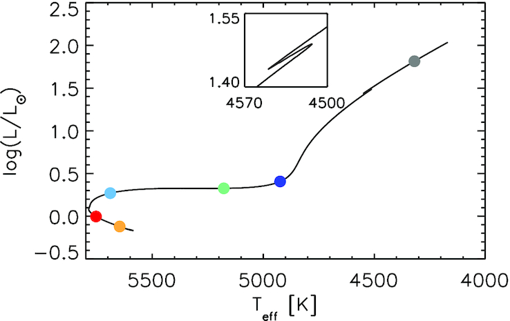
Fig.1: Herzsprung–Russell (H–R) diagram of a track with solar composition computed with MESA. The inset shows a zoom of the red giant branch bump (RGB bump). Figure from Hekker et al. (2020).
As summarised by Hekker et al. (2020), the RGB bump is believed to appear when the hydrogen shell burns through the mean molecular weight discontinuity left behind by the deepest extent of the convection zone. At this discontinuity, the amount of hydrogen available for burning increases and consequently there is a re-adjustment of the internal structure. This re-adjustment phase could explain the bump. However, Christensen-Dalsgaard (2015) showed that the burning shell only reaches the mean molecular weight discontinuity at the minimum luminosity. Hence, this picture cannot explain the luminosity maximum of the bump completely. Furthermore, it is known that the exact shape of the bump depends on the constituents of the models such as the hydrogen profile, as shown by, e.g. Cassisi,Salaris & Bono (2002).
In this minilab, you will therefore investigate the underlying microphysics (in particular, the specific entropy and its temporal gradient) that drives these phenomena using MESA and thereby reproduce the work of Hekker et al. (2020).
What you’ll learn
The primary purpose of this minilab is to get you more familiar with some topics in MESA beyond the absolute basics, including:
- Starting a project from a given test case and changing inlist controls
- Computing a few additional parameters and adding new history columns using
run_star_extras.f90 - Customizing
pgstar
Using this Guide
If you’re new to Fortran, here is a short document with some examples. Don’t let yourself get hung up by the Fortran; quickly ask your classmates and the TAs for help!
Every task comes with a hint and/or an answer. However, if you have prior experience with MESA, do attempt to complete the task on your own. The complete solution is available here.
Section 2: Getting Started
Task 2.1: Create your working directory for this minilab. It could be something like Much of this should be familiar already; here’s how you create your working directory and then change into that directory: The mkdir -p command is used to create a directory, including any necessary parent directories. This means that if the parent directory does not exist, mkdir -p will create it automatically.~/MESASS2025/Day4.
Note: you may also choose to place the working directory somewhere other than your home directory.Answer 2.1
mkdir -p ~/MESASS2025/Day4
cd ~/MESASS2025/Day4
Task 2.2: We have prepared and provided the test case for you. Discuss with your team members and choose a particular stellar mass to work with from here (local copy), download the corresponding Minilab1_xpxx.zip into the ~/MESASS2025/Day4 directory, unpack, and enter this work directory.
Links to all start directories
Answer 2.2
unzip Minilab1_xpxx.zip
cd Minilab1_xpxx
You are now ready to start the run!
Note
The rest of the guide demonstrates the particular case of a solar mass star; expect differences in numbers and plots depending on the stellar mass you’re working with. At the end of this lab, we will compare the different evolutionary tracks computed as a function of stellar mass across the room!
Task 2.3: Compile and run the provided work directory.
This directory evolves a star from the start of the RGB bump upto the end of the RGB bump. Confirm that you can compile and run it. Two default PGPLOT windows (Hertzsprung-Russell Diagram and temperature-density profille) should appear.
Answer 2.3
In your main work directory, run
./mk
./rn
This was a test run to ensure everything works fine for you; you do not need to complete the run at this point. When the two windows with plots appear, you may terminate the run using Ctrl + C.
Warning
It might take some time for the plots to appear, especially if OMP_NUM_THREADS has been set to 2; don’t kill the run before the plots appear.
Using inlists
You’re now familiar that MESA/star currently has five inlist sections: star_job, eos, kap, controls and pgstar, each containing the options for a different aspect of MESA.
Task 2.4: List the contents of your working directory and identity the number of inlists you see.Answer 2.4
Task 2.5: Open the prepared inlist_project and answer the following questions: (i) where does the model start its run from? (ii) what is the terminating condition used? (iii) what is the metallicity of the model computed? This example is for the case of
, check how the numbers vary for your particular case.
&star_job
	! begin with saved model
	load_saved_model = .true.
	load_model_filename = 'start_RGBB.mod'

	! save a model at the end of the run
	save_model_when_terminate = .true.
	save_model_filename = 'end_RGBB.mod'

	! display on-screen plots
	pgstar_flag = .true.

	pause_before_terminate=.true.

/ !end of star_job namelist

&eos
  ! eos options
  ! see eos/defaults/eos.defaults

/ ! end of eos namelist


&kap
  ! kap options
  ! see kap/defaults/kap.defaults
  use_Type2_opacities = .true.
  Zbase = 0.02

/ ! end of kap namelist

&controls
	! starting specifications
	initial_mass = 1.0 ! in Msun units
	initial_z = 0.02

	energy_eqn_option = 'eps_grav'

	log_L_upper_limit = 1.54

	!control output
	history_interval = 1
/ ! end of controls namelist
Answer 2.5
(i) The inlist_project loads a saved model called start_RGBB.mod that was pre-computed to save on computation time and start its run from that particular stage of evolution.
(ii) The run stops when the terminating condition of the upper limit of logL reaches 1.54. Different stopping conditions are provided under “! when to stop” in $MESA_DIR/star/defaults/controls.defaults.
(iii) The metallicity is Z=0.02. Note that Zbase is the base metallicity for the opacity tables, typically set to the same initial metallicity of the model, initial_z.
Tip
If you’re working on a slower machine, consider setting mesh_delta_coeff = 2.0d0 and time_delta_coeff = 2d0 in the &controls section of the inlist_project. A larger value in both increases the max allowed deltas and decreases the number of grid points, thereby reducing the run time.
Section 3: Using Run Star Extras
To customize run_star_extras.f90, navigate to the src directory that resides within your working directory and open run_star_extras.f90 in your text editor of choice. The stock version of run_star_extras.f90 is quite boring. It “includes” another file which holds the default set of routines.
include 'standard_run_star_extras.inc'The routines defined in the included file are the ones we will want to customize. Because we want these modifications to apply only to this working copy of MESA, and not to MESA as a whole, we want to replace this include statement with the contents of the included file.
Task 3.1: Delete the aforementioned include line and insert the contents of
$MESA_DIR/include/standard_run_star_extras.incin its entirety into run_star_extras.f90.
Hint 3.1
Answer 3.1: The partial run_star_extras.f90 solution is available here.
Task 3.2: Check that the code compiles and execute a test run to ensure everything works fine for you. Once the plots appear, you may terminate the run using Ctrl + C.
Answer 3.2
Navigate back to your main work directory and run:
cd ..
./clean && ./mk
./rn
If it doesn’t compile, double check that you cleanly inserted the file and removed the include line.
Note
Every time you make a change to run_star_extras.f90, remember to re-compile, otherwise the changes won’t be incorporated in your run.
Since run_star_extras.f90 was already introduced in the Day 2 Morning Session in considerable depth, we will now go straight to modifying it for our science test case.
Section 3.1: Studying the evolution of the RGB bump feature
One of our primary goals is to study the evolution of (i) the location of the base of the convection zone, (ii) the peak of the burning, and (iii) the mean molecular weight discontinuity around the RGB bump. Plotting these with mass coordinate and radius coordinate will reproduce Fig. 4 of Hekker et al. (2020) as shown below:
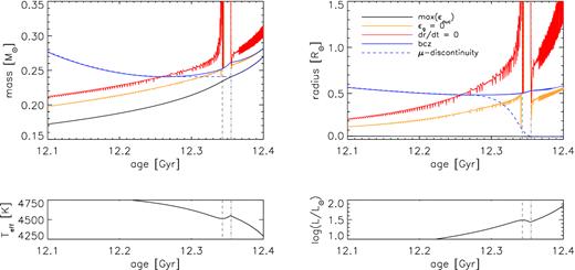
Fig.2: Top: the evolution around the bump of the location of the base of the convection zone, the peak of the burning, and the mean molecular weight discontinuity as a function of mass coordinate (left), and radius coordinate (right). Bottom: effective temperature (left) and luminosity (right) as a function of age. The vertical grey-dashed and dash–dotted lines indicate the age of the maximum luminosity and minimum luminosity of the bump feature, respectively. Figure from Hekker et al. (2020).
The base of the convection zone
Task 3.3: Output the mass coordinate at the base of the convection zone in your history.data by uncommenting the appropriate parameter in the history_columns.list.
Hint 3.3a
Hint 3.3b
Task 3.4: Output the radius coordinate at the base of the convection zone in your history.data by uncommenting the appropriate parameter in the history_columns.list.
Hint 3.4
Answer 3.3 and 3.4: At this point, your history_columns.list should look like this.
Task 3.5: While you’re at it, check if there exists default history columns for peak of the burning or the mean molecular weight in history_columns.list.
Answer 3.5: They don’t! Thankfully, we can customise our run_star_extras.f90 to compute additional parameters and add them as new history columns in the history.data file.
The peak of the burning
The goal here is to identify the zone (k) in the interior of the stellar structure where the nuclear burning (eps_nuc) is maximum and thereby find the mass and the radius corresponding to that zone.
Before making any changes to the run_star_extras.f90, take a quick look to identify where additional history columns may be added. The default looks as follows:
integer function how_many_extra_history_columns(id)
         integer, intent(in) :: id
         integer :: ierr
         type (star_info), pointer :: s
         ierr = 0
         call star_ptr(id, s, ierr)
         if (ierr /= 0) return
         how_many_extra_history_columns = 0
    end function how_many_extra_history_columns


subroutine data_for_extra_history_columns(id, n, names, vals, ierr)
         integer, intent(in) :: id, n
         character (len=maxlen_history_column_name) :: names(n)
         real(dp) :: vals(n)
         integer, intent(out) :: ierr
         type (star_info), pointer :: s
         ierr = 0
         call star_ptr(id, s, ierr)
         if (ierr /= 0) return

         ! note: do NOT add the extras names to history_columns.list
         ! the history_columns.list is only for the built-in history column options.
         ! it must not include the new column names you are adding here.


    end subroutine data_for_extra_history_columns
Tip
- Declare all new variables BEFORE the
ierr = 0statement in thedata_for_extra_history_columnssubroutine. - Add the new parameters to be computed and the new history columns AFTER the
if (ierr /= 0) returnstatement in thedata_for_extra_history_columnssubroutine. - Remember to update the right number in
how_many_extra_history_columns = 0as and when you add additional history columns in thehow_many_extra_history_columnsfunction.
Task 3.6: Compute the mass of the zone (in solar units) where the nuclear burning is at its maximum value and add it as a new column in your history.data.
Hint 3.6a
k=maxloc(s% eps_nuc, dim=1)
Hint 3.6b
Hint 3.6c
Hint 3.6d
Hint 3.6e
At this point, the partial solution to your run_star_extras.f90 file should look like this:
integer function how_many_extra_history_columns(id)
         integer, intent(in) :: id
         integer :: ierr
         type (star_info), pointer :: s
         ierr = 0
         call star_ptr(id, s, ierr)
         if (ierr /= 0) return
         how_many_extra_history_columns = 1
    end function how_many_extra_history_columns


subroutine data_for_extra_history_columns(id, n, names, vals, ierr)
         integer, intent(in) :: id, n
         character (len=maxlen_history_column_name) :: names(n)
         real(dp) :: vals(n)
         integer, intent(out) :: ierr
         type (star_info), pointer :: s
         integer :: k
	 real(dp) ::mass_max_eps_nuc

         ierr = 0
         call star_ptr(id, s, ierr)
         if (ierr /= 0) return

         k=maxloc(s% eps_nuc, dim=1)
    	 mass_max_eps_nuc = s% m(k)/Msun

         ! note: do NOT add the extras names to history_columns.list
         ! the history_columns.list is only for the built-in history column options.
         ! it must not include the new column names you are adding here.

         names(1) = "mass_max_eps_nuc"
	 vals(1) = mass_max_eps_nuc

    end subroutine data_for_extra_history_columns
Task 3.7: After making changes to the run_star_extras.f90, always check that the code compiles.
Answer 3.7
./clean && ./mkTask 3.8: Compute the radius of the zone (in solar units) where the nuclear burning is at its maximum value and add it as a new column in your history.data.
Hint 3.8a
Hint 3.8b
At this point, the partial solution to your run_star_extras.f90 file should look like this:
integer function how_many_extra_history_columns(id)
         integer, intent(in) :: id
         integer :: ierr
         type (star_info), pointer :: s
         ierr = 0
         call star_ptr(id, s, ierr)
         if (ierr /= 0) return
         how_many_extra_history_columns = 2
    end function how_many_extra_history_columns


subroutine data_for_extra_history_columns(id, n, names, vals, ierr)
         integer, intent(in) :: id, n
         character (len=maxlen_history_column_name) :: names(n)
         real(dp) :: vals(n)
         integer, intent(out) :: ierr
         type (star_info), pointer :: s
         integer :: k
	 real(dp) ::mass_max_eps_nuc, radius_max_eps_nuc

         ierr = 0
         call star_ptr(id, s, ierr)
         if (ierr /= 0) return

         k=maxloc(s% eps_nuc, dim=1)
    	 mass_max_eps_nuc = s% m(k)/Msun
         radius_max_eps_nuc = s% r(k)/Rsun

         ! note: do NOT add the extras names to history_columns.list
         ! the history_columns.list is only for the built-in history column options.
         ! it must not include the new column names you are adding here.

         names(1) = 'mass_max_eps_nuc'
	 vals(1) = mass_max_eps_nuc

         names(2) = 'radius_max_eps_nuc'
	 vals(2) = radius_max_eps_nuc

    end subroutine data_for_extra_history_columns
Answer 3.6 and 3.8: The partial run_star_extras.f90 solution is available here.
Task 3.9: After making changes to the run_star_extras.f90, always check that the code compiles.
Answer 3.9
./clean && ./mkThe mean molecular weight discontinuity
We will now include a new Fortran subroutine locdiscontinuity in the run_star_extras.f90 to identify the location of discontinuities in the mean molecular weight profile (with respect to the hydrogen abundance, X) of a stellar model. These discontinuities are important indicators of nuclear burning shells, convective boundaries, or mixing events in stellar evolution.
Task 3.10: Compute the mass and the radius at the location of the mean molecular weight discontinuity.
Hint 3.10: If you’d like to attempt on your own, please do so. However, since this is a little advanced, we have added the answer directly for your ease. Here is the snippet of how your run_star_extras.f90 should look like:
...
!calculate location of mean molecular weight discontinuity
      subroutine locdiscontinuity(id,nz,sdisc,sdiscdif)
          integer, intent(in) :: id, nz
          integer, intent(out) :: sdisc
          real(dp), intent(out) :: sdiscdif
          real(dp) :: x(nz), dif(nz-1)
          integer :: ierr, xs, xsb,k
          type (star_info), pointer :: s
          ierr = 0
          call star_ptr(id, s, ierr)
          if (ierr /= 0) return

          x = s% X(:nz)
          dif = x(:size(x)-1)-x(2:)
          k = maxloc(s% eps_nuc(:nz), dim=1)
          xsb = k
          sdisc=maxloc(dif, dim=1)
          sdiscdif=maxval(dif)

          end subroutine locdiscontinuity


integer function how_many_extra_history_columns(id)
         integer, intent(in) :: id
         integer :: ierr
         type (star_info), pointer :: s
         ierr = 0
         call star_ptr(id, s, ierr)
         if (ierr /= 0) return
         how_many_extra_history_columns = 4
    end function how_many_extra_history_columns

subroutine data_for_extra_history_columns(id, n, names, vals, ierr)
         integer, intent(in) :: id, n
         character (len=maxlen_history_column_name) :: names(n)
         real(dp) :: vals(n)
         integer, intent(out) :: ierr
         type (star_info), pointer :: s
         integer :: k, z, nz, sdisc
         real(dp) ::mass_max_eps_nuc, radius_max_eps_nuc, disc

         ierr = 0
         call star_ptr(id, s, ierr)
         if (ierr /= 0) return

          k=maxloc(s% eps_nuc, dim=1)
          mass_max_eps_nuc = s% m(k)/Msun
          radius_max_eps_nuc = s% r(k)/Rsun

         ! note: do NOT add the extras names to history_columns.list
         ! the history_columns.list is only for the built-in history column options.
         ! it must not include the new column names you are adding here.

          names(1) = 'mass_max_eps_nuc'
          vals(1) = mass_max_eps_nuc
          names(2) = 'radius_max_eps_nuc'
          vals(2) = radius_max_eps_nuc

          nz = s% nz
          names(3) = 'mdisc'
          names(4) = 'rdisc'

         call locdiscontinuity(id,nz,sdisc,disc)
         vals(3) = s% m(sdisc)/(Msun)
         vals(4) = s% r(sdisc)/(Rsun)
    end subroutine data_for_extra_history_columns
...
Explanation 3.10
An explanation of the Fortran subroutine locdiscontinuity is included here:
!=======================================================================
! Subroutine: locdiscontinuity
! Purpose: Identify locations and magnitudes of composition discontinuities
!          in a stellar model, often associated with hydrogen abundance (X).
!=======================================================================
subroutine locdiscontinuity(id, nz, sdisc, sdiscdif)

  ! Input arguments
  integer, intent(in) :: id         ! Model identifier
  integer, intent(in) :: nz         ! Number of zones

  ! Output arguments
  integer, intent(out) :: sdisc   ! Index of strongest outer-layer discontinuity
  real(dp), intent(out) :: sdiscdif ! Magnitude of strongest outer-layer discontinuity

  ! Local variables
  real(dp) :: x(nz)                 ! Composition profile (e.g. hydrogen abundance)
  real(dp) :: dif(nz-1)             ! Backward differences between mesh points
  real(dp) :: max_eps_h_m
  integer :: ierr, xs, xsb, k
  type (star_info), pointer :: s   ! Pointer to stellar structure data

  ierr = 0
  call star_ptr(id, s, ierr)        ! Get pointer to star data
  if (ierr /= 0) return             ! Exit if pointer setup fails

  x = s% X(:nz)                     ! Load hydrogen abundance profile
  dif = x(:size(x)-1) - x(2:)       ! Compute differences between adjacent zones

  k = maxloc(s% eps_nuc(:nz), dim=1) ! Find zone of peak nuclear energy generation
  xsb = k                            ! (used as proxy for peak H burning)

  sdisc = maxloc(dif(:xsb-1), dim=1) ! Max discontinuity above burning zone
  sdiscdif = maxval(dif(:xsb-1))     ! Its magnitude

end subroutine locdiscontinuity

!=======================================================================
! Extracting physical information from discontinuities
!=======================================================================
call locdiscontinuity(id, nz, sdisc, disc)

vals(3) = s% m(sdisc) / (Msun)
! Mass (in solar units) of the outer-layer discontinuity

vals(4) = s% r(sdisc) / (Rsun)
! Radius (in solar units) of the outer-layer discontinuity
Answer 3.10: The partial run_star_extras.f90 solution is available here.
Task 3.11: Once again, after making changes to the run_star_extras.f90, check that the code compiles.
Answer 3.11
./clean && ./mkGreat work! You have now included most of the parameters that are required to reproduce Fig. 4 of Hekker et al. (2020).
Section 3.2: The variation of the ‘gravothermal’ energy generation rate with age
As mentioned earlier, this lab aims to probe the importance of entropy in RGB evolution. In stars, the rate of change of specific entropy is proportional to , the ‘gravothermal’ energy generation rate. Therefore, we also want to study the variation of at the base of the convection zone as a function of age around the evolution of the RGB bump and thereby reproduce Fig. 6 of Hekker et al. (2020) as shown below:
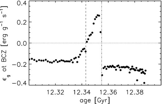
Fig.3: The value of at the base of the convection zone as a function of age. The vertical dashed and dash–dotted lines indicate the stellar ages of the luminosity maximum and luminosity minimum of the bump, respectively. The horizontal dotted line indicates zero. Figure from Hekker et al. (2020).
In Section 3.1, we had already seen how to include the mass and the radius coordinates at the base of the convection zone. We only had to uncomment the history column names in the history_columns.list since they are computed as default history columns. However, this holds clue to how one may compute new additional parameters at the base of the convection zone. To look at how the mass and the radius ordinates were computed at the base of the convection zone, open the file:
$MESA_DIR/star/private/history.f90and search for cz_bot_mass or cz_bot_radius.
Tip
The default history columns are defined in the $MESA_DIR/star/private/history.f90 file. If you inspect that file, you can use their definitions as templates for writing your own new history columns.
Task 3.12: Compute
at the base of the convection zone cz_eps_grav and add it as a new column in your history.data.
Hint 3.12a
Hint 3.12b
Here is the snippet of code that can be used in the run_star_extras.f90:
 if (s% largest_conv_mixing_region /= 0) then
                z = s% mixing_region_bottom(s% largest_conv_mixing_region)
                cz_eps_grav = s% eps_grav_ad(z)% val
             end if
Hint 3.12c: Here is the snippet of how your run_star_extras.f90 should look like:
...
integer function how_many_extra_history_columns(id)
         integer, intent(in) :: id
         integer :: ierr
         type (star_info), pointer :: s
         ierr = 0
         call star_ptr(id, s, ierr)
         if (ierr /= 0) return
         how_many_extra_history_columns = 5
    end function how_many_extra_history_columns

subroutine data_for_extra_history_columns(id, n, names, vals, ierr)
         integer, intent(in) :: id, n
         character (len=maxlen_history_column_name) :: names(n)
         real(dp) :: vals(n)
         integer, intent(out) :: ierr
         type (star_info), pointer :: s
         integer :: k, z, nz, sdisc
         real(dp) ::mass_max_eps_nuc, radius_max_eps_nuc, disc, cz_eps_grav

         ierr = 0
         call star_ptr(id, s, ierr)
         if (ierr /= 0) return

          k=maxloc(s% eps_nuc, dim=1)
          mass_max_eps_nuc = s% m(k)/Msun
          radius_max_eps_nuc = s% r(k)/Rsun

        if (s% largest_conv_mixing_region /= 0) then
                z = s% mixing_region_bottom(s% largest_conv_mixing_region)
                cz_eps_grav = s% eps_grav_ad(z)% val
             end if

         ! note: do NOT add the extras names to history_columns.list
         ! the history_columns.list is only for the built-in history column options.
         ! it must not include the new column names you are adding here.

          names(1) = 'mass_max_eps_nuc'
          vals(1) = mass_max_eps_nuc
          names(2) = 'radius_max_eps_nuc'
          vals(2) = radius_max_eps_nuc

          nz = s% nz
          names(3) = 'mdisc'
          names(4) = 'rdisc'

         call locdiscontinuity(id,nz,sdisc,disc)
         vals(3) = s% m(sdisc)/(Msun)
         vals(4) = s% r(sdisc)/(Rsun)

         names(5) = 'cz_eps_grav'
         vals(5) = cz_eps_grav
    end subroutine data_for_extra_history_columns
...
Answer 3.12: The final run_star_extras.f90 solution is available here.
Task 3.13: As always, after making changes to the run_star_extras.f90, check that the code compiles.
Answer 3.13
./clean && ./mkNow that you have all the parameters, you are essentially ready to start the run! If you’re short on time, you may grab the final inlist_pgstar here and jump straight to Section 5. However, if you’re interested and have time, let’s customise the inlist_pgstar in the next section for a better understanding of how the stellar structure/interiors change as the star evolves around the RGB bump.
Section 4: Customizing pgstar [BONUS EXERCISE]
pgstar is a built-in feature of MESA that allows for real-time graphical insight into how your model is evolving. While the plots it generates are usually not suitable for publication, being able to “see” your model evolve can be an invaluable tool in developing intuition and diagnosing issues. Additionally, you can easily string frames of pgstar output into a movie after a simulation, which is great for presentations and group meetings!
pgstar is comprised of several building blocks that we can sort into several [slightly-overlapping] categories.
History Plots
Plots that show one or two quantities from the history output plotted against a monotonically-increasing quantity, like star_age or model_number. These quantities must all be saved in history.data, and the resolution will depend on how often data is written to history.data.
Profile Plots
Plots that show one or two quantities that could be output in profiles against another profile quantity, often pressure, mass coordinate, or radius. Note that these do not need to be in profile.columns since they do not need to persist over multiple steps.
Special Plots
A collection of “one-off” plots with special capabilities. Examples include Kippenhahn diagrams, echelle diagrams, a nuclear network diagram, and a temperature-density profile. These can often be customized to a degree, but they are not as flexible as profile and history plots.
Text Summaries
Grids of name/value pairs that show scalar values associated with the current timestep. Examples include model number luminosity, and helium core mass. No graphics here; just text.
Most often, you’ll deal with a grid or dashboard that contains many individual single- or multi-panel plots and/or text summaries arranged into a single window. We’ll explore this next.
Goal: In this section, in addition to the default Hertzsprung-Russell Diagram and temperature-density profile, we will also visualise the variation of the specific entropy, mean molecular weight, density, pressure, temperature and in the stellar interiors as a function of mass fraction.
Task 4.1: Open the inlist_pgstar in your favourite editor and turn the HR_win_flag and TRho_Profile_win_flag to false to prevent their individual PGPLOT windows.
Answer 4.1
 HR_win_flag = .false.
 TRho_Profile_win_flag = .false.
Task 4.2: Include the first profile panel in the inlist_pgstar to display specific entropy, mean molecular weight, density as a function of mass fraction.
Answer 4.2
 ! Profile Panels 1

  Profile_Panels1_title = 'Profile Panels'
  Profile_Panels1_xaxis_name = 'mass'
  Profile_Panels1_xmin = 0
  Profile_Panels1_xmax = 1

  Profile_Panels1_show_mix_regions_on_xaxis = .false.
  Profile_Panels1_yaxis_name(1) = 'entropy'
  Profile_Panels1_yaxis_name(2) = 'mu'
  Profile_Panels1_yaxis_name(3) = 'logRho'

  Profile_Panels1_other_yaxis_name(1) = ''
  Profile_Panels1_other_yaxis_name(2) = ''

  Profile_Panels1_num_panels = 3
Task 4.3: Include the second profile panel in the inlist_pgstar to display
, temperature and pressure as a function of mass fraction.
Hint 4.3
 ! Profile Panels 2

    Profile_Panels2_title = 'Profile Panels'
    Profile_Panels2_xaxis_name = 'mass'
    Profile_Panels2_xaxis_reversed = .false.
    Profile_Panels2_xmin = 0
    Profile_Panels2_xmax = 1

    Profile_Panels2_show_mix_regions_on_xaxis = .false.
    Profile_Panels2_yaxis_name(1) = 'eps_grav'
    Profile_Panels2_yaxis_name(2) = 'logT'
    Profile_Panels2_yaxis_name(3) = 'logP'
    Profile_Panels2_num_panels = 3
Task 4.4: Include a few important parameters as part of the text block in the pgstar.
Answer 4.4
 ! Text Summary 1

  Text_Summary1_name(1,1) = 'model_number'
  Text_Summary1_name(2,1) = 'log_star_age'
  Text_Summary1_name(3,1) = 'log_dt'
  Text_Summary1_name(4,1) = 'log_L'
  Text_Summary1_name(5,1) = 'log_Teff'
  Text_Summary1_name(6,1) = 'log_R'
  Text_Summary1_name(7,1) = 'log_g'
  Text_Summary1_name(8,1) = 'log_surf_cell_P'

  Text_Summary1_name(1,2) = 'star_mass'
  Text_Summary1_name(2,2) = 'log_abs_mdot'
  Text_Summary1_name(3,2) = 'he_core_mass'
  Text_Summary1_name(4,2) = 'co_core_mass'
  Text_Summary1_name(5,2) = 'h_rich_layer_mass'
  Text_Summary1_name(6,2) = 'he_rich_layer_mass'
  Text_Summary1_name(7,2) = ''
  Text_Summary1_name(8,2) = ''

  Text_Summary1_name(1,3) = 'log_cntr_T'
  Text_Summary1_name(2,3) = 'log_cntr_Rho'
  Text_Summary1_name(3,3) = 'log_center_P'
  Text_Summary1_name(4,3) = 'center h1'
  Text_Summary1_name(5,3) = 'center he4'
  Text_Summary1_name(6,3) = 'center c12'
  Text_Summary1_name(7,3) = 'center n14'
  Text_Summary1_name(8,3) = 'center o16'

  Text_Summary1_name(1,4) = 'log_Lnuc'
  Text_Summary1_name(2,4) = 'log_Lneu'
  Text_Summary1_name(3,4) = 'log_LH'
  Text_Summary1_name(4,4) = 'log_LHe'
  Text_Summary1_name(5,4) = 'log_LZ'
  Text_Summary1_name(6,4) = 'num_zones'
  Text_Summary1_name(7,4) = 'num_retries'
  Text_Summary1_name(8,4) = ''
Task 4.5: Now combine all the grid information to activate the customised pgstar dashboard. The parameters are adopted from $MESA_DIR/star/defaults/pgstar.defaults.
Answer 4.5
 ! Grid1,information to combine all plots into Grid1

  Grid1_win_flag = .true.
  Grid1_win_width = 12
  Grid1_win_aspect_ratio = 0.55
  Grid1_xleft = 0.06
  Grid1_xright = 0.95
  Grid1_ybot = 0.08
  Grid1_ytop = 0.92
  Grid1_title = ''

  Grid1_num_cols = 3
  Grid1_num_rows = 8
  Grid1_num_plots = 5

  Grid1_plot_name(1) = 'TRho_Profile'
  Grid1_plot_row(1) = 1
  Grid1_plot_rowspan(1) = 3
  Grid1_plot_col(1) = 1
  Grid1_plot_colspan(1) = 1
  Grid1_plot_pad_left(1) = 0
  Grid1_plot_pad_right(1) = 0.05
  Grid1_plot_pad_top(1) = 0
  Grid1_plot_pad_bot(1) = 0.1
  Grid1_txt_scale_factor(1) = 0.7

  Grid1_plot_name(2) = 'HR'
  Grid1_plot_row(2) = 4
  Grid1_plot_rowspan(2) = 3
  Grid1_plot_col(2) = 1
  Grid1_plot_colspan(2) = 1
  Grid1_plot_pad_left(2) = 0
  Grid1_plot_pad_right(2) = 0.05
  Grid1_plot_pad_top(2) = 0.03
  Grid1_plot_pad_bot(2) = 0
  Grid1_txt_scale_factor(2) = 0.7

  Grid1_plot_name(3) = 'Profile_Panels1'
  Grid1_plot_row(3) = 1
  Grid1_plot_rowspan(3) = 6
  Grid1_plot_col(3) = 2
  Grid1_plot_colspan(3) = 1
  Grid1_plot_pad_left(3) = 0.04
  Grid1_plot_pad_right(3) = 0.03
  Grid1_plot_pad_top(3) = 0
  Grid1_plot_pad_bot(3) = 0
  Grid1_txt_scale_factor(3) = 0.65

  Grid1_plot_name(4) = 'Text_Summary1'
  Grid1_plot_row(4) = 7
  Grid1_plot_col(4) = 1
  Grid1_plot_rowspan(4) = 2
  Grid1_plot_colspan(4) = 3
  Grid1_plot_pad_left(4) = -0.08
  Grid1_plot_pad_right(4) = 0
  Grid1_plot_pad_top(4) = 0.08
  Grid1_plot_pad_bot(4) = -0.05
  Grid1_txt_scale_factor(4) = 0.25

  Grid1_plot_name(5) = 'Profile_Panels2'
  Grid1_plot_row(5) = 1
  Grid1_plot_rowspan(5) = 6
  Grid1_plot_col(5) = 3
  Grid1_plot_colspan(5) = 1
  Grid1_plot_pad_left(5) = 0.06
  Grid1_plot_pad_right(5) = 0.02
  Grid1_plot_pad_top(5) = 0.0
  Grid1_plot_pad_bot(5) = 0
  Grid1_txt_scale_factor(5) = 0.65

  Grid1_file_flag = .true.
  Grid1_file_dir = 'png'
  Grid1_file_prefix = 'rgbb_'
  Grid1_file_interval = 1
  Grid1_file_width = -1
  Grid1_file_aspect_ratio = -1
Your final inlist_pgstar should look like this.
Section 5: Putting it all together
You’re now finally ready to start the run!
Task 5.1: Start the run
Answer 5.1
./rnThe customised PGPLOT window should look something like this:
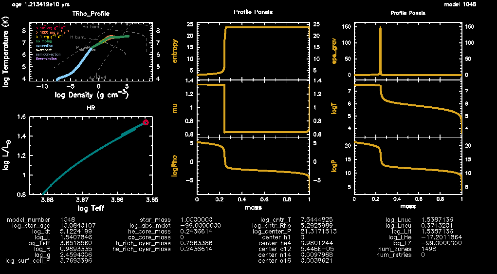
Fig.4: The PGPLOT dashboard exhibiting the HR diagram, temperature-density plot and additional profile panels for a track with solar composition.
The complete run should take around 6 minutes on 6 threads. While the model evolves, here’s what to look out for on your PGPLOT window. Locate the profile panel (top right) that shows the variation of as a function of the stellar structure- the zone that exhibits the peak is where we have the H-shell burning. The layers interior to this zone represent the core while those outside represent the stellar envelope. This reference point now makes it easy to study how all the other stellar parameters vary in the stellar structure (core vs envelope) as the model evolves. Note that for the profile panels, while the profile shape itself doesn’t seem to change, the values definitely do- keep an eye out for the -axes values as the model evolves.
After the run terminates, you’re ready to plot and reproduce the figures of Hekker et al. (2020).
Tip
At the end of the run, take a look at the HR diagram. Was the stopping condition actually applied?
Note
If you were unable to complete the run or would like to verify your history.data output file, you may grab the pre-computed output history files corresponding to your chosen mass from here.
Task 5.2: Use this Google Colab notebook
(local copy)
to upload your history.data and plot (i) the evolution around the RGB bump of the location of the base of the convection zone, the peak of the burning, and the mean molecular weight discontinuity as a function of mass coordinate and radius coordinate and compare your output plot with Fig. 4 of Hekker et al. (2020).
Warning
The axes limits in the Google Colab notebook are customised for the case of ; please change axes limits according to your chosen stellar mass to “zoom in” for better visualisation. There may be numerical artefacts in certain cases which result in a horizontal line at ; you may safely ignore that.
Answer 5.2
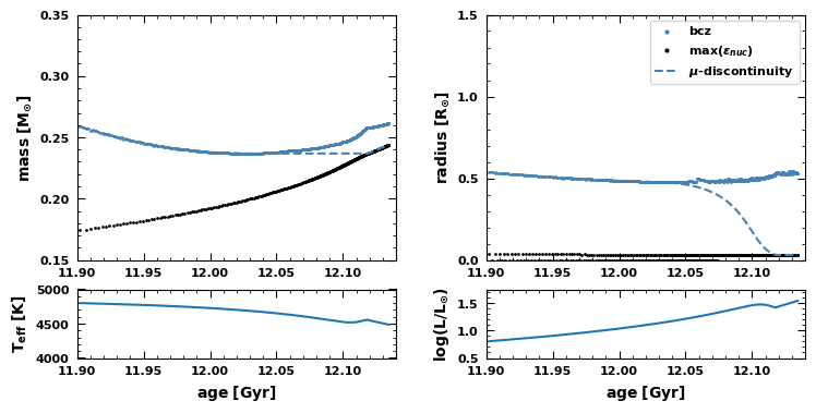
Fig.5: The evolution around the bump of the location of the base of the convection zone, the peak of burning and the mean molecular weight discontinuity as a function of mass and radius coordinate.
Task 5.3: Using the same Google Colab notebook, plot the variation of at the base of the convection zone as a function of age and compare your output plot with Fig. 6 of Hekker et al. (2020).
Answer 5.3
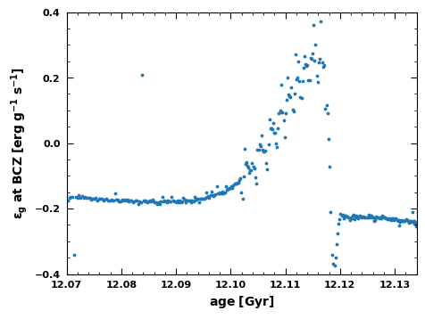
Fig.6: The variation of at the base of the convection zone as a function of age.
Task 5.4: For this task, each team will upload one history.data. Rename your history.data as history_1pxx.data, reflecting the stellar mass you’ve been working with and post it on the Day 4 channel of Mattermost. A TA will plot the evolutionary tracks of all stellar masses computed to compare the difference in the evolution of the RGB bumps across the room using this Google Colab notebook
(local copy)
.
Answer 5.4
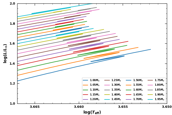
Fig.7: The evolution of the RGB bumps for different stellar masses.
Acknowledgements: This guide includes some material from previous MESA Summer Schools, in particular, from https://jschwab.github.io/mesa-2021/ and https://billwolf.space/projects/mesa-ss-2022/.