Monday MaxiLab 1: Modeling core overshooting in main-sequence stars

In this lab, you will learn how to set up a MESA model from scratch, monitor the run, customize its output and choose reasonable values for model parameters. Our science case is focused on the effects of core overshooting on the core of main-sequence stars.

As a maxilab, this lab will take two 1.5h sessions. Each session is organized in three sections, structured as below with an estimate of the time you are expected to spend on each. Please do not hesitate to ask your TA and/or the other people at your table for assistance if you notice you are falling behind.

Session 1

Setting up your MESA work directory [~20 min.]

Copying the default work dir

We will start from the default MESA work directory and slowly build it up until we have a fleshed-out main-sequence model. Copy the default work directory into a new folder called lab1 and navigate into said folder:

cp -r $MESA_DIR/star/work lab1
cd lab1

Do a quick ls to check what is included in this default work directory. You’ll see a number of executables, namely clean, mk, re and rn. The subdirectories make and src contain the Makefile and extra code to include, but you don’t have to look into that today. For now, let’s take a look at the inlists inlist, inlist_pgstar and inlist_project. The term inlist refers to MESA’s standard Fortran namelist file that launches a simulation. It’s a plain text file where you group configuration variables into sections (namelists) These files describe what you want MESA to do. In particular MESA will always look for inlist. Using your favorite text editor, take a look at what is in inlist.

What this inlist essentially does is redirect MESA to the other two inlist files for all the real content, with inlist_project containing most of the fields describing how the MESA run should go and inlist_pgstar describing what visuals MESA should produce. For now, focus on inlist_project.

Basic initial parameters

Let’s start with a very simple main-sequence model of a star with an initial mass of 5 solar masses and metallicity of 0.014 with some strong step-wise mixing due to core overshooting. To do so, open inlist_project and find and change the following parameters to the given values:

initial_mass = 5d0
initial_z = 0.014d0

The opacity table MESA uses depends on the reference metallicity, defined by Zbase under the &kap namelist. For consistency, you should set Zbase to the same value as initial_z:

Zbase = 0.014d0

Adding overshooting

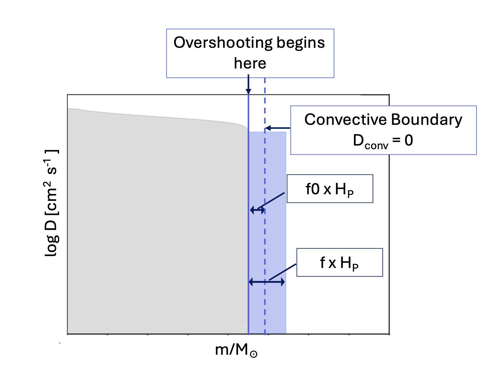
Next, to add the core overshooting, we need to add in some new fields, shown below. As you plug this into your inlist, have a look at the questions below.

overshoot_zone_type(1) = 'burn_H'
overshoot_zone_loc(1) = 'core'
overshoot_bdy_loc(1) = 'top'
overshoot_scheme(1) = 'step'
overshoot_f(1) = 0.30d0
overshoot_f0(1) = 0.005d0

Question: The first three overshoot_ fields describe where the overshooting should take place. Go into the MESA documentation and look up what each of these fields means.

Question: Where should you add these fields?

Bonus Question: Why does each overshoot field in our example have that (1) at the end?

Termination conditions

Before you run your model, you should consider when the model is terminated. Since we want to simulate the main-sequence evolution, we should place our stopping condition at the terminal age main-sequence (TAMS). Look under ! when to stop in &controls of your inlist_project.

There are two conditions that can trigger the model to end. The first is

Lnuc_div_L_zams_limit = 0.99d0
stop_near_zams = .true.

which is designed to stop the model at the zero-age main-sequence (ZAMS), that it defines as the point where 99% of the energy released comes from nuclear reactions. As we seek to model the main-sequence, we obviously do not want the run to end around the ZAMS. Therefore, disable stop_near_zams by setting:

stop_near_zams = .false.

The second condition is meant to stop the model around the TAMS.

xa_central_lower_limit_species(1) = 'h1'
xa_central_lower_limit(1) = 1d-3

Question: How does the default inlist_project define the TAMS?

For our purposes today, it will be interesting to go a little bit further. Therefore, change the lower limit on ${}^1$ H to $10^{-6}$ :

xa_central_lower_limit_species(1) = 'h1'
xa_central_lower_limit(1) = 1d-6

Running the model

Run your model to the TAMS by cleaning any executables in your work directory using

./clean
./mk
./rn

As your model runs, you will notice that MESA writes heaps of numbers to your terminal. After a while, two panels with constantly changing plots pop up. They show the evolutionary track of your model on a Hertzsprung-Russell diagram and one the internal temperature and density profiles. These help you keep a close eye on your model and can help you identify problems and potential improvements.

For now, let’s focus on the terminal output. One important field for our purposes is the central hydrogen fraction (H_cntr), which tells you how far along the main-sequence evolution your model is. Note that it initially changes extremely slowly. This is because MESA starts with a very small time step which gradually increases, as shown by the lg_dt_yrs field, the base 10 logarithm of the time step expressed in years.

Some optimisations

Before running our main model, let’s make two adjustments to speed up the MESA run:

MESA starts by creating a pre-main-sequence model (before nuclear burning begins) and by default performs 300 relaxation steps to ensure it’s stable. For our educational purposes, we can reduce this to save time by adding to the &star_job section of your inlist_project:

pre_ms_relax_num_steps = 100

MESA also starts with very tiny time steps after the pre-main sequence model has been created and relaxed. We can tell it to use larger initial steps, by adding the following under &star_job:

set_initial_dt = .true.
years_for_initial_dt = 1d0

These adjustments will help our model run faster, especially during the early phases. In your future research, you’d want to carefully test how these parameters affect your specific science case, but for this lab, these settings are fine.

If you want to (and are on schedule), you can briefly run your model again by entering ./rn in your terminal to test whether your changes to the inlist did what they are supposed to.

If you got stuck and cannot get your inlist to run, you can find a functional inlist with all the changes described above here , so you can continue with limited delay. Be sure to rename inlist_project1 to inlist_project!

Modifying the input physics and saving your final model [~20 min.]

Mass loss

inlist_project is currently mostly empty, meaning most settings are using MESA’s default values. You should always check whether these are appropriate for your models. As an example, massive stars can loose a fair amount of mass through winds.

Check what the default wind mass loss is. You can find this in the documentation of &controls to see what the default wind mass loss is. You could also look through the default values in the MESA code inside $MESA_DIR/star/defaults/ (controls.defaults in this case), though the website documentation is easier to navigate if you don’t know the name of the relevant fields yet.

You will see in the documentation that there is a wealth of wind mass loss schemes available, all of which can be scaled up or down by a constant factor. Each scheme is appropriate in particular regimes of the surface temperature, composition, etc. The so-called Dutch scheme attempts to merge some of these schemes into a cohesive whole. Add it into your inlist_project without scaling.

hot_wind_scheme = 'Dutch'
cool_wind_RGB_scheme = 'Dutch'
Dutch_scaling_factor = 1d0

The mixing-length parameter

MESA uses the mixing-length theory (MLT) to describe the transport by convection. This theory relies on the scaling factor ${\alpha }_{MLT}$ , which expresses for how many pressure scale heights a convective fluid parcel maintains its properties. Typically values range between 1 and 3. You should check what MESA’s default value of this ${\alpha }_{MLT}$ parameter is.

When you are working on your real science cases, you should test a few different values for this ${\alpha }_{MLT}$ to gain an understanding of its effects. However, to save some time in this lab, we will stick to just one value, namely 1.8. Add this into your inlist_project under &controls:

mixing_length_alpha = 1.8d0

Saving the final model

In the other labs today, you will learn how to run models that continue after the main-sequence evolution. Instead of re-running the main-sequence evolution every time you tweak a setting, we can tell MESA to save a model at the end of a main-sequence run.

The default inlist explicitly tells MESA not to save the model. Find the fields below and change them to:

save_model_when_terminate = .true.
! Give a name to the model file to be saved including your parameter values, e.g.
! 'M{your_M}_Z{your_Z}_fov{your_f_overshoot}_f0ov{your_f0_overshoot}.mod'
save_model_filename = 'M5_Z0014_fov030_f0ov0005_TAMS.mod'

Running the updated model

Despite how much you already added into your inlist_project, there are still many empty headers. Indeed, when building an inlist for your real science cases, you should still look into your opacity tables, atmosphere settings, equation of state, spatial and temporal resolution, and much more. However, for the sake of time, we’ll stop here.

Now let’s run the model again! To do so, enter

./rn

into your terminal.

If you got stuck and cannot get your inlist to run, you can find a functional inlist with all the changes described above here , so you can continue with limited delay. Be sure to rename inlist_project2 to inlist_project!

Customising output [~30 min.]

Upgrading the pgstar plots

Now let’s turn to these animated plots, often called the pgstar plots. These are incredibly useful in understanding what is going on in your model while its running, helping you spot potential problems early. Therefore, it is worthwhile to customize your pgstar panels to show those quantities that are the most important to your work. To this end, MESA has a bunch of prepared windows you can easily add by adding one flag to your inlist_pgstar. You can find these and how to edit your inlist_pgstar in this documentation page.

For this lab, we have prepared a specialized inlist_pgstar for you. **Download that inlist_pgstar ** here and move it into your MESA work directory. Make sure to name the file inlist_pgstar!

Run your model again to see what the new pgstar plots look like.

For some of you, this new panel may be very small or bigger than your screen. This is because the width of the pgstar window is dependent on your system and the size of your screen. If the panel is too large or small for you, open inlist_pgstar, find the two lines shown below near the top of the inlist and edit these values until the panel looks nice.

Grid1_win_width = 10
Grid1_win_aspect_ratio = 0.7

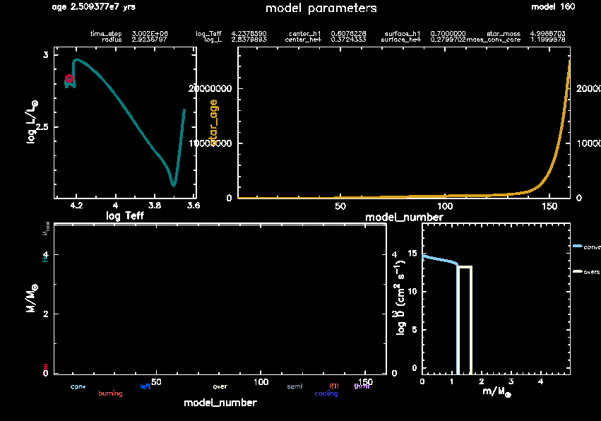
Understanding this pgstar window

We have merged all the plots in one panel for a better overview. We also included some key quantities at the top, similar to MESA’s terminal output.

The plots are:

• Top left: The Hertzsprung-Russell diagram (HRD),
• Top right: History panel showing model number on the x-axis and age on the y-axis.
  (This is often used as a proxy for age since model number increments regularly during evolution),
• Bottom right: The mixing panel,
• Bottom left: This is a mysterious, mostly-empty panel. We’ll get back to that empty panel later.

We’ll refer to the “history plot” (top right) throughout the lab, so keep that panel in mind.

pause_before_terminate = .true.

For now, turn to that mixing panel in the bottom right and ponder these questions:

Question: What is the mixing panel showing exactly? What does the color of each line indicate?

Bonus Question: Why do we plot the model number on the x-axis instead of, say, the stellar age?

Customizing MESA’s output data

In your pgstar window, look at the plot in the top right corner. This panel is showing how model properties change over time, currently using model number as the x-axis (In many cases, the absolute age of the star doesn’t matter. Since age correlates closely with model number, and model number is easier to interpret, we often use it as a proxy). Since we’re studying core overshooting effects, we’d like to modify this panel to show the evolution of the core mass instead of the default value.

To customize what’s displayed in MESA plots, we first need to understand what data is being tracked. When MESA runs, it creates a LOGS directory containing two main types of output files:

• history.data: Records global stellar properties at each timestep
• profile*.data: Captures the star’s internal structure at specific timesteps

Open LOGS/history.data with a text editor. After the header information, you’ll see a list of column names around line 6. These are all the quantities MESA has been tracking during your run.

To add more quantities to track, we need to customize the history columns list. First, we need to copy the default history column list to our work folder:

cp $MESA_DIR/star/defaults/history_columns.list my_history_columns.list

Open my_history_columns.list and take a minute to explore the wealth of available output options. The file is organized by category, with comments explaining most variables. This gives you a comprehensive view of what MESA can track.

For our overshooting study, we’re interested in the stellar core properties. The convective core mass is already included in the defaults. Let’s add the star’s radius to the history output by finding and uncommenting the radius field in the appropriate section.

Once you have uncommented the relevant lines, you need to tell MESA that you want to include the output columns in my_history_columns.list. To do so, add the following line into your inlist_project under &star_job:

history_columns_file = 'my_history_columns.list'

Finally, let’s consider how often MESA writes this history output.

Bonus Question: How often does MESA write its history output by default?

As we don’t need that many history columns, it’s reasonable to write them at every step. Do so by setting in your &controls:

history_interval = 1

Configuring the History Plot

Now let’s customize the History Panel in the pgstar window. This panel shows how stellar properties evolve over time.

1. Open inlist_pgstar in your text editor
2. Find the section that defines the History Panel (search for “History_Panels1”)
3. Change the y-axis to display the convective core mass:

History_Panels1_yaxis_name(1) = 'mass_conv_core'

This will show how the convective core mass evolves throughout the star’s main sequence lifetime.

To enable more advanced plotting features like the Kippenhahn diagram (which shows the internal structure evolution), we need to tell MESA to track additional data. Open my_history_columns.list and find and uncomment the following options:

mixing_regions 20
burning_regions 20

These settings tell MESA to track up to 20 distinct mixing and nuclear burning regions within the star, which enables the creation of Kippenhahn diagrams and other detailed evolutionary plots.

Run your model briefly to confirm your pgstar window now displays the updated plot configuration.

Bonus Task – Profile Data

While history files track global properties over time, profile files capture the star’s internal structure at specific moments. These are essential for examining how variables change with radius inside the star. Copy over the default profile column list.

cp $MESA_DIR/star/defaults/profile_columns.list my_profile_columns.list

To study mixing processes in the stellar interior, uncomment these fields:

• log_D_mix - the diffusion coefficient for mixing
• mixing_type - identifies which mixing process is active in each zone

After modifying this file, tell MESA to use your custom profile columns by adding to your inlist_project under &star_job:

profile_columns_file = 'my_profile_columns.list'

Bonus Question: By default, MESA only saves a profile every 50 model steps. This might miss important evolutionary phases. How could you increase this frequency?

Bonus Question: How many profiles can MESA write over the course of a run? Why might you want to limit it?

If you got stuck and cannot get your inlist to run, you can find a functional inlist with all the changes described above here , so you can continue with limited delay. Be sure to rename inlist_project3 to inlist_project! You can also find the completed inlist pgstar here, the completed history columns list here, and the completed profile columns list here.

Bonus Task – Movies

ls -lh png/

cd png

images_to_movie '*.png' evolution.mp4

images_to_movie "*.png" evolution.mp4

Session 2

Adapting the input parameters and assessing their importance [~15 min.]

You now know how to navigate your work directory and build up a main-sequence model. That’s great! However, so far we have limited ourselves to simply adding in pre-chosen parameter values, choices of tables etc. In real scientific applications, you should always consider the impact of these settings, for instance by trying a few different values. In particular, there are a number of numerical schemes and uncertain physical parameters for which you should think carefully about the appropriate value. You already encountered some of these today, namely the mixing length parameter ${\alpha }_{MLT}$ and convective overshooting.

In this session, we’ll explore the impact of overshooting in your model. The plan is that everyone gets a unique set of overshooting parameters, initial mass and initial metallicity to try out. You will then compare the results of these parameter settings to the model you produced in session 1. Meanwhile, we will collect some basic results from everyone’s models and examine the correlations between different parameters together.

Bonus Question: Overshooting in MESA starts overshoot_f0 scale heights into the convection zone. If you use step overshooting, the overshooting ends overshoot_f scale heights above the start of overshooting, after which the overshoot mixing goes to zero. But how does MESA define where the overshooting stops when you use exponential overshooting, which never goes all the way to zero?

Picking new initial parameters

Go into this spreadsheet (mirror) and put your name next to one set of parameters to claim it as yours. Modify your inlist accordingly.

Since there are more parameter sets available than there are students, you can test different parameters if time allows. However, the main focus should be on completing this task and fully understanding it. Additionally, the bonus tasks in this lab involve running this set of parameters in a batch.

If you selected the ’no overshoot’ scheme from the spreadsheet, you should leave the overshoot scheme as an empty string, i.e.

overshoot_scheme(1) = ''

If you selected the ’exponential’ scheme, you should consider where the overshoot region ends. As the mixing strength decreases exponentially, it approaches zero far away from the core-envelope boundary. As such, past a certain point, the mixing is so small as to become meaningless. Therefore, MESA stops the overshoot mixing when the mixing coefficient drops below 100 cm${}^2$ /s. This is quite a high lower limit, so reduce it by setting in your &controls :

overshoot_D_min = 1d-2

Preserving Your Previous Results

We’ll make two adjustments to keep our work organized. After selecting your parameter set from the spreadsheet, modify the save_model_filename in your inlist_project file to reflect these specific parameters:

save_model_filename = 'M{mass}_Z{metallicity}_{scheme}_fov{fov}_f0ov{f0}.mod'

For example, if you selected a 15 $M_{\odot }$ star with $Z=0.014$ , exponential overshooting with $f_{\text{ov}}=0.01$ and $f_0=0.001$ , your filename would be:

save_model_filename = 'M15_Z0014_exponential_fov001_f0ov0001.mod'

MESA normally writes all history and profile data to a directory called LOGS/. To keep these outputs separate from your previous run, we’ll direct MESA to use a different output directory. Add the following to your inlist_project under the &controls section:

log_directory = 'LOGS_M{mass}_Z{metallicity}_{scheme}_fov{fov}_f0ov{f0}'

Using the same example parameters as above:

log_directory = 'LOGS_M15_Z0014_exponential_fov001_f0ov0001'

This keeps all your runs organized with descriptive names that make it easy to identify which parameters were used for each model.

Running your model again

Now run your model again. Keep a close eye on your pgstar plots, particularly the mixing panel. Compare it with those of the other people at your table.

Collecting the TAMS output

After your model finishes running, we’ll extract key parameters at the Terminal Age Main Sequence (TAMS).

Open the final history.data file in your new LOGS directory with a text editor. The TAMS is represented by the final line in this file - this is where the central hydrogen has been depleted to the threshold we set (1d-6) and the run was ended.

From this final line, record the following values in the second page of the spreadsheet:

• log_Teff (logarithm of effective temperature)
• log_L (logarithm of luminosity in solar units)
• mass_conv_core or he_core_mass (depending on which is available)
• conv_mx1_top_r (if you uncommented this)
• star_age/1e6 (to convert to Myr)

These values will allow us to analyze how different overshooting parameters affect stellar evolution.

If you got stuck and cannot get your inlist to run, you can find a functional inlist with all the changes described above here , so you can continue with limited delay. Be sure to rename inlist_project4 to inlist_project! You will still have to update the parameters and output filenames and directory according to your parameter set though. Ask your TA for assistance with that.

Bonus Task – Plotting MESA output

Now let’s wrap up this lab by reading your MESA output in using Python and making some custom plots.

For an introduction into utilising python as an analysis tool, see bonus_tasks/python_analysis.

Bonus Task – Batch Parameter Studies with MESA

If you’ve completed the main lab activities and have time remaining, explore the automated parameter study framework in the bonus_tasks/ directory. This framework enables systematic exploration of overshooting effects across a grid of stellar model parameters.

For complete documentation and additional analysis tools, see bonus_tasks/.