Joel Ong Courtney Crawford Lea Schimak Meng Sun
MESA School 2025
July 25, 2025
We will learn about how to do asteroseismology with mesa — this is not mainly a course about asteroseismology.
We will provide some background throughout, however.
For the uninitiated, we have prepared a quick primer on it to go with the online tutorials.
We recommend further reading resources at the end of these slides.
physics of stellar interiors
quantitative
astronomy & astrophysics
Asteroseismology is our
only direct probe of
stellar interiors
(in the electromagnetic spectrum)
(Zero-Age) Main Sequence
(core hydrogen-burning)
Red Giant Branch
(shell hydrogen-burning)
Red Clump/Horizontal Branch \(\to\)
(core helium-burning)
(RHD simulations courtesy of Joel D. Tanner)

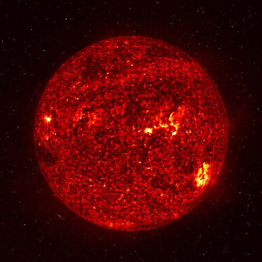
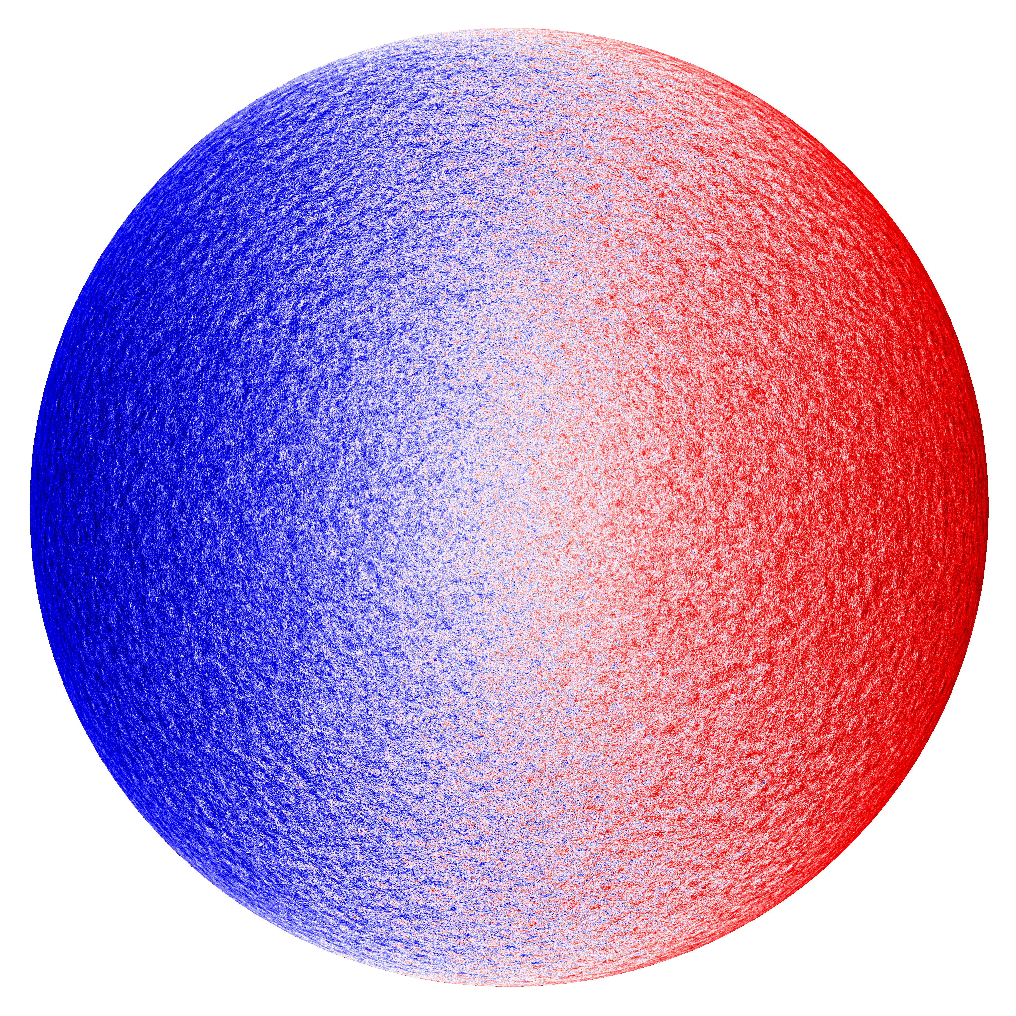
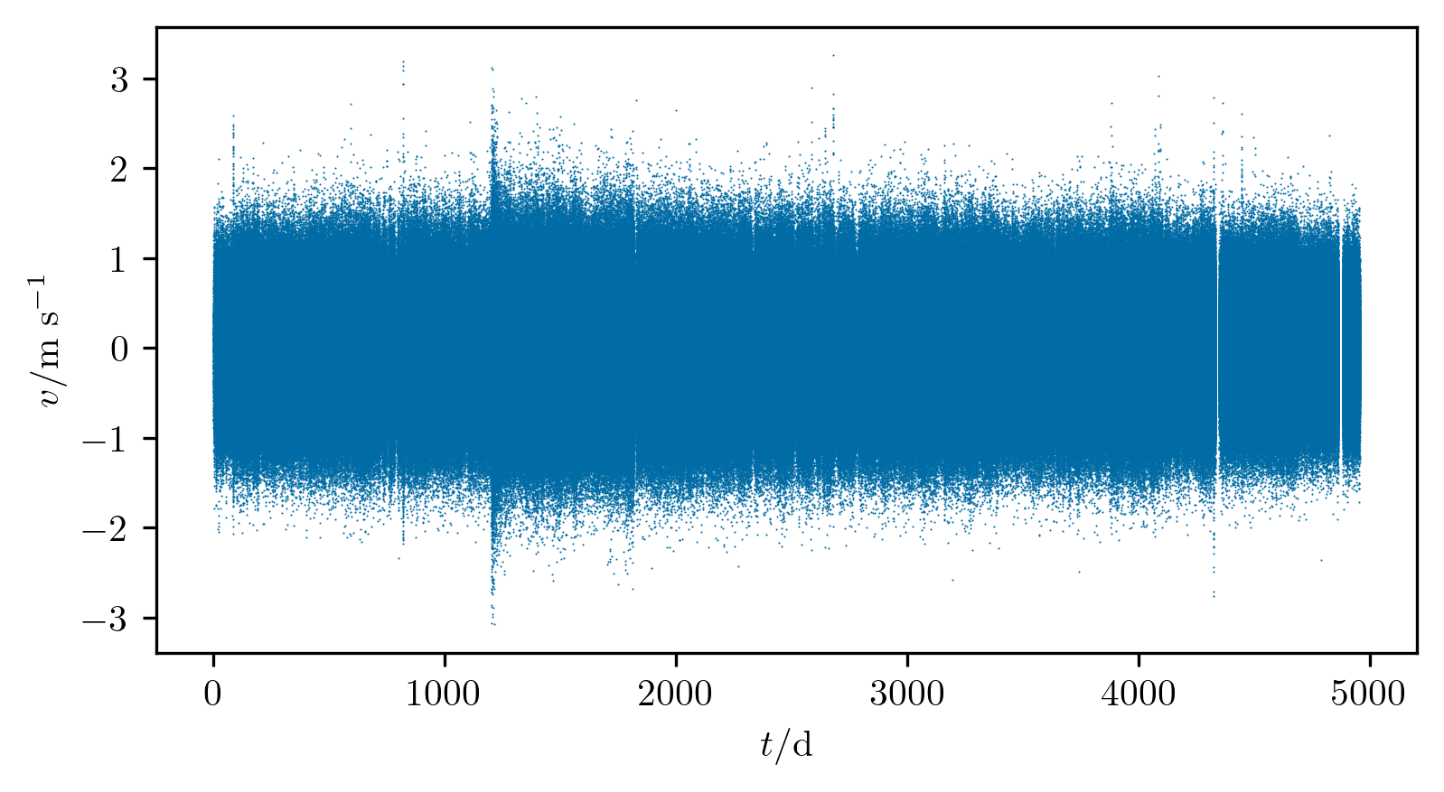
\(\ell = 0\) MDI Doppler velocities
\[ \begin{aligned} {\Delta\nu} & \sim 1/t_\text{cross} \sim \sqrt{M/R^3}\\ {\nu_{\text{max}}} &\sim{g/c_s} \sim {M/R^2\sqrt{T_\text{eff}}} \end{aligned} \]
\[V_\text{osc} \sim L / M\]
Each one of these peaks
tells us the frequency of
a normal mode of oscillation (i.e. the natural
frequency of a standing wave).
These mode frequencies
are determined by
the internal structure and dynamics
of the medium in which these standing waves
propagate.
Today, we will examine how one might calculate the mode frequencies of a rotating red giant.
Data: \(y_\text{obs} \in Y\)
Models: \(x_i \in X\);\[F: X \to Y\]
Best-fitting model: \[x = \mathop{\mathrm{argmax}}_{x_j \in X}\ \mathcal{L}\left(x_j\right)\]
\[F: \underbrace{\left(M, t, Y_0, Z_0, \alpha_\text{mlt}, \ldots\right)}_{x \in X} \mapsto \underbrace{\left(L, T_\text{eff}, [\text{M/H}], \log g, \ldots\right)}_{y \in Y}\]

\[ \color{darkorange} \to \Delta\nu, \nu_{\text{max}}, \left\{\nu_{n,l}\right\} \]

A stable release of gyre is included with mesa, which we will use today.
More up-to-date versions can always be found on GitHub — but we will not be using them today.
Rich Townsend maintains a phpBB forum for gyre user questions.
Upon successful compilation, run gyre by calling it as
\[\left<\Omega\right>_g\]
\[\left<\Omega\right>_p\]
(\(\leftarrow\) proxy for age)
Radiative core contracts dramatically off main sequence
\(\implies\) core spins up (if
conserving angular momentum)
inlist files
and run_star_extras.f from the Lab 1 website —\[\huge {\partial^2 \over \partial t^2}f(t, \mathbf{x}) = c_s^2 \nabla^2 f(t, \mathbf{x})\]
\[\huge -\omega^2 \hat{f}(\omega, \mathbf{k}) = -c_s^2 |\mathbf{k}|^2 \hat{f}(\omega, \mathbf{k})\]
Dispersion relation: \[\boxed{\huge \omega^2 = c_s^2 |\mathbf{k}|^2}\]
\[\huge {\partial^2 \over \partial t^2}f = \left(c_s^2 \nabla^2 - \omega^2_\text{ac}(\mathbf{x})\right) f\]
\[\huge \underbrace{-\nabla^2 f}_{\equiv k^2f} = -\left(\omega^2 - \omega^2_\text{ac}(\mathbf{x}) \over c_s^2\right) f\]
Wave propagates where \(k^2(r,
\omega) > 0\),
and decays where \(k^2(r, \omega)
< 0\).
\(\left<\Omega\right>_1 = {\int_{X_1} \Omega(x) k \mathrm d x \over \int_{{X_1}} k \mathrm d x}\)
\(\left<\Omega\right>_2 = {\int_{X_2} \Omega(x) k \mathrm d x \over \int_{{X_2}} k \mathrm d x}\)
\[\begin{aligned}{\partial^2 \over \partial t^2} \rho \boldsymbol \xi & = {\color{blue}\nabla (\rho c_s^2\nabla \cdot \boldsymbol \xi)} + {\color{red}\nabla(\boldsymbol \xi \cdot \rho \mathbf g) - \rho \mathbf g \nabla \cdot \boldsymbol \xi} - {\color{orange}\mathbf g (\boldsymbol \xi \cdot\nabla \rho)} \\&-\color{gray}{4\pi G \rho \nabla \int {1 \over 4\pi |\mathbf x - \mathbf x'|}\nabla \cdot (\rho(\mathbf x') \boldsymbol \xi(\mathbf x'))\ \mathrm d^3 x'}.\end{aligned}\]
\[- \omega^2 \rho \boldsymbol \xi = \left({\color{blue}-c_s^2\mathbf{k k}^T} + {\color{red}i(\mathbf{k}\mathbf{g}^T - \mathbf{g}\mathbf{k}^T)} + {\color{orange}{g\over \rho}{\mathrm d \rho \over \mathrm d r} \mathbf{e_r}\mathbf{e_r}^T} - {\color{gray}{4\pi G\rho \mathbf{k k}^T\over |\mathbf{k}|^2}} \right)\rho \boldsymbol \xi\]
(full derivation in PDF notes)
\[- \omega^2\begin{bmatrix}\xi_r \\ \xi_h\end{bmatrix} = \left({\color{blue}-c_s^2\mathbf{k k}^T} + {\color{red}i(\mathbf{k}\mathbf{g}^T - \mathbf{g}\mathbf{k}^T)} + {\color{orange}{g\over \rho}{\mathrm d \rho \over \mathrm d r} \mathbf{e_r}\mathbf{e_r}^T} \right)\begin{bmatrix}\xi_r \\ \xi_h\end{bmatrix}\]
\[\omega^2 \begin{bmatrix}\xi_r \\ \xi_h\end{bmatrix} = \begin{bmatrix} {\color{blue}c_s^2k_r^2} - {\color{orange}{g \over \rho} {\mathrm d \rho \over \mathrm d r}} & {\color{blue}c_s^2k_r k_h} + {\color{red} i g k_h} \\ {\color{blue}c_s^2k_r k_h} - {\color{red} i g k_h} & {\color{blue}c_s^2k_h^2}\end{bmatrix}\begin{bmatrix}\xi_r \\ \xi_h\end{bmatrix}\]
The eigenvalues \(\omega^2\) are roots of the characteristic equation
\[\begin{aligned}{\color{blue}c_s^2 k_r^2} &= \omega^2\left(1 - {{\color{blue}c_s^2 k_h^2}\over \omega^2}\right)\left(1 - {{\color{orange} N^2} \over \omega^2}\right) - \left({\color{red}c_s \over \Gamma_1 H_p}\right)^2.\end{aligned}\]
where \(N^2 = g \left({1 \over \Gamma_1 P} {\mathrm d P\over \mathrm d r} - {1 \over \rho} {\mathrm d \rho\over \mathrm d r}\right)\) — also recall that for spherical harmonics, \(k_h^2 = \ell(\ell + 1) / r^2\)
\[{c_s^2 k_r^2 \sim \omega^2 \left(1 - {{\color{blue} S_\ell}^2 \over \omega^2}\right)\left(1 - {{\color{darkorange}N}^2 \over \omega^2}\right)}\]
\[\small N^2 = {- g}\left.{\partial \log \rho \over \partial s}\right|_P{\mathrm d s \over \mathrm d r}\] entropy gradient (\(=0\) in CZ)
\[\small S_\ell^2 = c_s^2 k_h^2 = {\ell(\ell+1) c_s^2 \over r^2}\] wave angular momentum
\[\Large \omega_-^2 \sim N^2 {k_h^2 \over |\mathbf{k}|^2}; \boldsymbol \xi \sim \begin{bmatrix}k_h \\ k_r\end{bmatrix} \perp \mathbf{k}\]
\[{\color{red} \omega_g < N, S_\ell}\]
\[\Large \omega_+^2 \sim c_s^2 |\mathbf{k}|^2; \boldsymbol \xi \sim \begin{bmatrix}k_r \\ k_h\end{bmatrix} \parallel \mathbf{k}\]
\[{\color{gray} \omega_p > S_\ell, N}\]
Pressure waves (p-modes)
propagate isotropically.
p-modes:
Characteristic overtone frequency spacing \(\Delta\nu\)
Buoyancy waves (g-modes)
propagate anisotropically.
g-modes:
Characteristic overtone period spacing \(\Delta\Pi_\ell\)
p-modes:
\[\large\boxed{\nu = \Delta\nu\left(n + {\ell \over 2} + \epsilon_p\right)}\]
\[\small\Delta\nu \sim \left(2 \int {\mathrm d r \over c_s}\right)^{-1}\]
g-modes:
\[\large\boxed{{1 \over \nu} = \Delta\Pi_\ell \left(n + {\ell \over 2} + \epsilon_{g, \ell}\right)}\]
\[\small\Delta\Pi_\ell \sim {2\pi^2 \over \sqrt{\ell(\ell+1)}}\left(\int {N \over r} \mathrm d r\right)^{-1}\]
\[\left(\text{f-modes: }\omega^2 = g k_h = \sqrt{\ell(\ell + 1)}\cdot{GM \over R^3}\right)\]
Suppose we wished to find \(\lambda\) and \(\psi\) satisfying \[ \left(-{\partial^2 \over \partial x^2} + V(x)\right)\psi(x) = \lambda \psi(x). \]
Discretisation: Let \(y_i \equiv \psi(x_i)\), \(V_{ij} \equiv V(x_i)\delta_{ij}\), and \(\left(\mathbf{D}\mathbf{y}\right)_i \sim \psi'(x_i)\). \[ \boxed{\LARGE\implies\left(-\mathbf{D}^2 + \mathbf{V}\right)\mathbf{y} = \lambda \mathbf{y}.} \]
If \(\left(-\mathbf{D}^2 + \mathbf{V} -
\lambda \mathbb{1}\right)\mathbf{y} = 0\), then \(\lambda\) must be
a root of the characteristic function \[\Large F(\lambda) =\det\left[-\mathbf{D}^2 +
\mathbf{V} - \lambda \mathbb{1}\right].\]
Suppose we wished to find \(\lambda\) and \(\psi\) satisfying \[ \left(-{\partial^2 \over \partial x^2} + V(x)\right)\psi(x) = \lambda \psi(x). \]
Discretisation: Let \(y_i \equiv \psi(x_i)\), \(V_{ij} \equiv V(x_i)\delta_{ij}\), and \(\left(\mathbf{D}\mathbf{y}\right)_i \sim \psi'(x_i)\). \[ \boxed{\LARGE\implies\left(-\mathbf{D}^2 + \mathbf{V}\right)\mathbf{y} = \lambda \mathbf{y}.} \]
&model, &osc,
&mode, &constants,
&rot
&num, &grid
&scan
namelist file&model to set file to the
stellar model of your choice:Power spectra of MDI dopplergrams
\[ \begin{aligned} {\Delta\nu_\odot} &\sim 135\ \mathrm{\mu Hz} \\ {\nu_{\text{max},\odot}} &\sim 3090\ \mathrm{\mu Hz} \end{aligned} \]
(roughly 5-minute oscillations)
p-mode frequencies satisfy \(\nu_{n\ell} \sim \Delta\nu\left(n + {\ell \over 2} + \epsilon_\ell(\nu)\right) + \mathcal{O}(1/\nu)\)
Stochastic,
broad-band
excitation


\[\begin{array}{c} {\scriptsize\text{Power}}\\ \big\uparrow \end{array}\]
\[\longrightarrow {\scriptsize\text{Frequency}}\]
(proxy for age \(\to\))
Mixed modes exhibit
avoided crossings
between underlying p- and
g-modes.
For \(\pi\) modes:
For \(\gamma\) modes:
&rot namelist&rot. However, if your stellar models
are rotating, these rotation rates can be used instead:Three quantum numbers \(n, l, m\): \[ \begin{aligned} \ell &= 0, 1, 2, \ldots \\ m &= -\ell, -\ell+1, \ldots, \ell-1, \ell \end{aligned} \]
Zonal (\(m = 0\))
Prograde sectoral
(\(m = +\ell\))
Retrograde sectoral
(\(m = -\ell\))
\[\begin{array}{c} {\scriptsize\text{Power}}\\ \big\uparrow \end{array}\]
\[\longrightarrow {\scriptsize\text{Frequency}}\]
An extra term appears in the momentum equation going as \[ {\mathrm D \mathbf v \over \mathrm d t} = \text{(other terms)} + \boxed{\boldsymbol \Omega \times \mathbf{v}}. \] We may account for how this changes the mode frequencies by
We replace \(\boldsymbol \Omega = \Omega \mathbf{e_z} \to (\boldsymbol \Omega \cdot \mathbf{e}_r) \mathbf{e}_r = \Omega \cos \theta \mathbf{e_r}\). This causes the pulsation problem to remain amenable to separation of variables.
Recall: this means solutions are of the general form, e.g.,
\(P(r, \theta, \varphi) = \tilde{P}(r)
\Theta(\theta) \Phi(\varphi)\).
By azimuthal symmetry, \(\Phi(\varphi) = e^{\mathrm{i} m \varphi}\) for integer \(m\).
Without rotation, the solution in the latitude coordinate, \(\Theta\), satisfies \[{\mathrm d \over \mathrm d \mu} \left({1 - \mu^2} {\mathrm d \over \mathrm d \mu} \Theta\right) - {m^2 \over (1 - \mu^2)} \Theta = \lambda \Theta.\]
This is Laplace’s equation with eigenvalues \(\lambda = \ell (\ell + 1)\) for integers \(\ell\).
With rotation, this becomes Laplace’s tidal equation: \[\left[{\mathrm d \over \mathrm d \mu} \left({1 - \mu^2 \over 1 - q^2 \mu^2} {\mathrm d \over \mathrm d \mu}\right) - {m^2 \over (1 - \mu^2)(1 - q^2 \mu^2)} + {m q (1 + q^2 \mu^2) \over (1 - q^2 \mu^2)^2}\right] \Theta = \lambda \Theta,\] with the spin parameter \(q = 2\Omega/\omega\).
Solutions are given by the Associated Legendre Polynomials, \(P_\ell^m(\cos \theta).\)
Solutions are given by the
Hough Functions, \(H_\ell^m(\cos
\theta, q).\)
p-modes:
\[\large\boxed{\nu = \Delta\nu\left(n + {\ell \over 2} + \epsilon_p\right)}\]
\[\nu \to \nu + m \left(1 - {1 \over 2 \left(\ell + {1 \over 2}\right)}{\Delta\nu \over \nu}\right){\Omega \over 2\pi}\]
g-modes:
\[\large\boxed{{1 \over \nu} = {\Delta\Pi_0 \over \sqrt{\ell (\ell + 1)}} \left(n + {\ell \over 2} + \epsilon_{g, \ell}\right)}\]
\[\nu \to \nu + m\left(1 - {1 \over \ell (\ell + 1)}\right){\Omega \over 2\pi}\]
Inertial modes \(\left(\text{e.g.}~\text{Rossby}~\text{modes, }\omega = -{2 \Omega m \over \ell(\ell + 1)}\right)\ldots\)
Mode mixing yields avoided crossings
between multiplet components of identical \(m\)
(cf. Mosser+ 2012, Ouazzani+ 2013, Deheuvels+ 2017)
Mode inertia \(I = \int r^2 \rho_0 \left(\xi_r^2 + \ell(\ell + 1) \xi_t^2\right) \mathrm d r.\)
For rotation in particular, \[\delta\omega \sim m \beta \int K(r)\Omega(r)\ \mathrm d r;\] \[\beta K(r) = {r^2 \rho_0 \over I} \left(\xi_r^2 + [\ell(\ell+1) - 1] \xi_t^2 - 2\xi_r \xi_t\right)\] (with \(K(r)\) normalised to unit integral)