Lab 1: Installing and using GYRE
Learning Goals
- Install GYRE
- Calculate a 1 Msun rotating MESA model for use with GYRE
- Calculate the JWKB estimators for rotation seen by g-modes and p-modes
MESA is distributed with two codes for stellar oscillations:
The calculations performed by the two are essentially equivalent, with the main tradeoff being between performance and ease of use. In this tutorial, we will restrict our attention to GYRE, which is much easier to get started with.
Installing GYRE
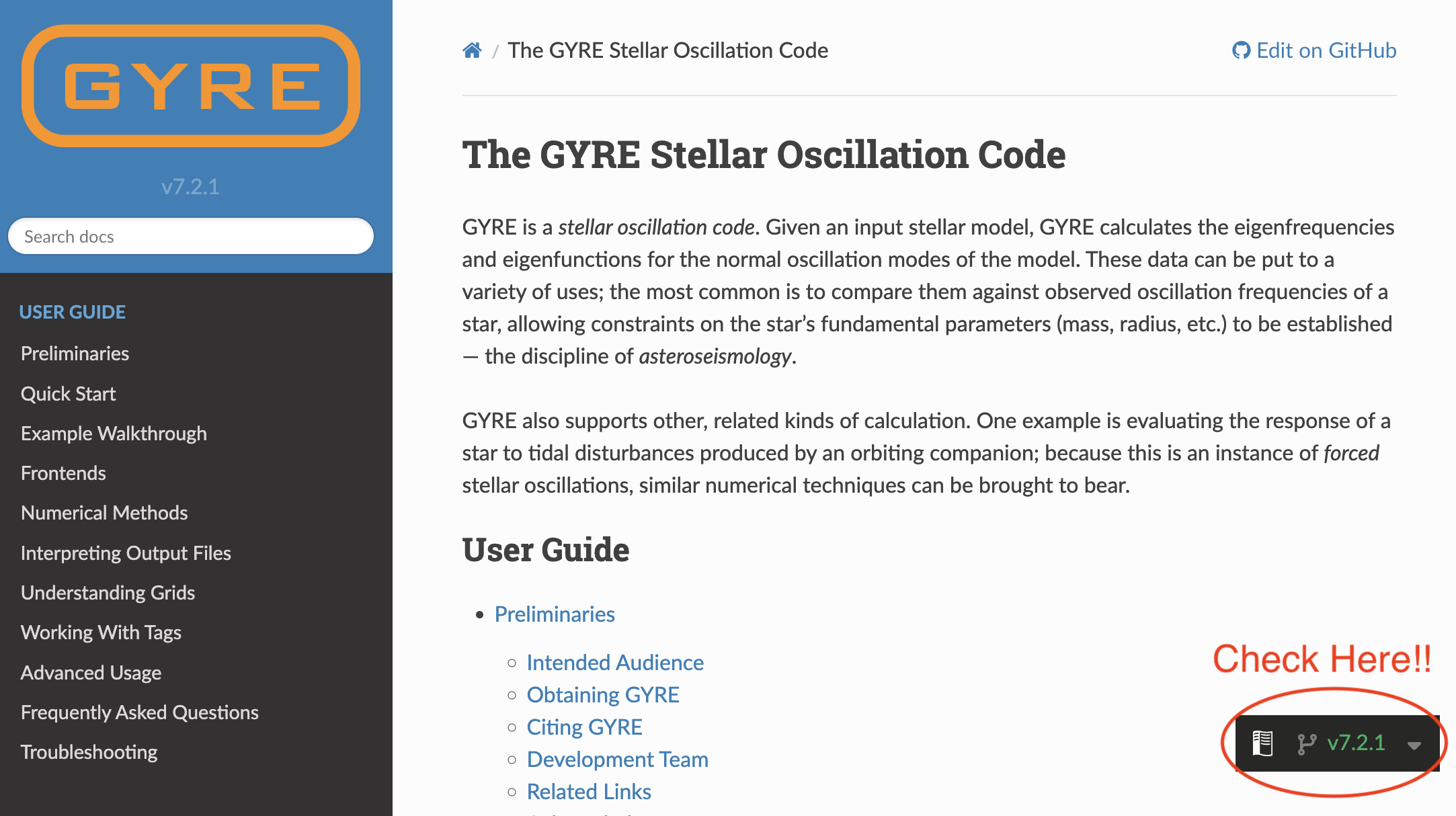
GYRE comes automatically packed in with your MESA installation. For MESA version 24.08.1, the shipped GYRE version is 7.2.1. However, GYRE has since updated to version 8.0. Be sure that you are viewing the docs for the correct version number of the GYRE version that you are using. For GYRE 7.2.1, the link to the documentation is here.
See the screenshot below to check for the correct GYRE version when viewing the docs. If you see “latest” or “stable” here, that indicates you are viewing version 8.0 (for now, until a new update comes out).
The GYRE Docs contains a tutorial for GYRE installation. However, since we are not installing GYRE from a tar file, we will slightly modify what is written in this guide. The instructions are copied below with explicit changes listed.
Extracting GYRE
We will not need to extract the GYRE source code from a tar file, as it is already extracted.
Set Environment Variables
Secondly, we will set the environment variable $GYRE_DIR equal to the following:
export GYRE_DIR=$MESA_DIR/gyre/gyre
Remember that this is best placed inside your shell’s RC file in your home directory (usually .bashrc or equivalent), similarly to when you first installed MESA. Don’t forget to source this file to apply the changes to your terminal window!
Compile
Now, we can follow the GYRE installation guide from this point. Go ahead and compile:
make -j -C $GYRE_DIR install
Test
Once that’s complete, it’s good practice to run the test suite to ensure nothing has gone wrong during the installation process:
make -C $GYRE_DIR test
Note
If all the tests read “…succeeded” then you are good to move on to the next step. If that’s not the case, ask your TA or a developer for help.
Create a rotating red giant star model
In today’s labs, we will be studying the oscillation frequencies of red giant stars and how those oscillations are affected by rotation. So, to start, we will need to generate a model of a red giant star that is rotating.
1: Download our template
First, extract all of the files from the template into a new working directory for your rotating star model. Call it whatever you like. Your working directory should have the following files in it.
>> tree .
.
├── ck
├── clean
├── history_columns.list
├── inlist
├── inlist_1M_star
├── inlist_pgstar
├── make
│   └── makefile
├── mk
├── profile_columns.list
├── re
├── rn
├── src
│   ├── run_star_extras.f90
│   └── run.f90
└── tams.mod

3 directories, 14 files
2: Update the template files
The files you’ve downloaded will be a template version of the files you need to run this lab. First we will need to add a few lines to the inlist that runs the star (inlist_1M_star).
&star_job
Notice that we are starting from a
TAMS model called tams.mod. That TAMS model is non-rotating, but this isn’t an issue for our rotating model. We initialize the rotation at TAMS in order to save time in the simulation. In your science, you should initialize rotation in a place that makes sense for the problem you are working on. For our purposes, this will be fine as we only care about rotation on the RGB phase.
We will initialize rotation in the &star_job portion of the inlist. There are many options in MESA for this (see docs here for an example). We will initialize our rotation as a solid body by setting an initial
which will be constant across the star.
For today’s set of labs, you will pick a rotation rate based on your table. These are all available in our google sheet for this lab. You will upload information from these labs to this sheet throughout the day. At each table, there will be four different nu_max values to choose from. We will use this value of nu_max as a proxy for the age of your rotating RGB star in this lab and the later ones. For now, decide in your group who will choose each value of nu_max and claim your model directly in the google sheet. In lab 2 and 3, the lower nu_max values will take slightly longer than others to run, so choose according to your computing speed if you need to.
| 📋 TASK |
|---|
| 1. Pick a rotation rate and nu_max value from the google sheet (local copy; nu_max will be used later on in the labs.) |
2. Add the following lines to the star_job portion of inlist_1M_star |
    new_rotation_flag = .true.
    change_rotation_flag = .true.
    change_initial_rotation_flag = .true.
    new_omega_div_omega_crit = ### ! INSERT YOUR ROTATION RATE HERE
    set_initial_omega_div_omega_crit = .true.
    set_omega_div_omega_crit = .true.
Note
In this lab, we have turned on rotation, but we have NOT turned on the flags corresponding to rotationally induced mixing or angular momentum transport. In your own science cases, you will need to make a choice about how you implement these two things.
controls
The only thing we’ll need to update in &controls is to ensure that MESA outputs the type of files needed for GYRE, and includes the correct parts of the star. These files are usually referred to as pulse_data in the MESA docs.
| 📋 TASK |
|---|
1. Add the relevant lines to the &controls portion of your inlist that will output GYRE files with each profile. These files should be in the GYRE format. Also make sure they include the atmosphere, the surface point, and should be in double point precision. |
ℹ️ HINT 1
ℹ️ SOLUTION
   write_pulse_data_with_profile = .true.
   add_atmosphere_to_pulse_data = .true.
   keep_surface_point_for_pulse_data = .true.
   add_double_points_to_pulse_data = .true.
   pulse_data_format = 'GYRE'
While you don’t need to change these, you should notice that we are running this model at low resolution (large mesh_delta_coeff and time_delta_coeff). Once again, you should choose this value to reflect your science question and convergence studies. We have chosen this value to prioritize running speed.
run_star_extras.f90
Since our star is rotating, we can calculate analytically the effect of rotation on the different types of oscillation modes (p-modes and g-modes) in the red giant star. These will be discussed further in Lab 3, but for now we should implement the calculation of them.
In the JWKB approximation, we have the following estimators for p-modes and g-modes, respectively:
Where
indicates the rotation rate (s% omega),
indicates the Brunt-Väisälä frequency (s% brunt_N) and
indicates the sound speed (s% csound). These estimators are, effectively, average values of of the rotation rate as sensed by p- and g-modes in a star.
We can easily add these estimators to the MESA output as a history file. We will outline the process below, since there are some fortran specifics you may not know, but feel free to go ahead and code up these equations now if you are confident in your fortran coding.
| 📋 TASK |
|---|
1. Edit the how_many_extra_history_columns section of your src/run_star_extras.f90 file to tell it we are going to add two new columns. |
ℹ️ SOLUTION
First, edit the function how_many_extra_history_columns to tell it we are going to add two new columns.
      integer function how_many_extra_history_columns(id)
        integer, intent(in) :: id
        integer :: ierr
        type (star_info), pointer :: s
        ierr = 0
        call star_ptr(id, s, ierr)
        if (ierr /= 0) return
        how_many_extra_history_columns = 2 !! change this line
      end function how_many_extra_history_columns
delta_omega_p
Lets start with
. To calculate this term, we will need to integrate over the whole star. In order to do this, we have included a function in the template src/run_star_extras.f90 file that is called integrate_r_ which is lifted straight from the GYRE utility functions. Notice the first line of this function:
function integrate_r_(x, y, mask) result(int_y)This indicates that we will need to input an array for x and y, and an optional argument called mask, and the function will return a number. Note that int_ means integrated, not an integer. In our case, x will be the array describing the radius of the star, which you can retrieve from the star pointer. The y array will be the integrand portion of the equations given above. For
you will not need a mask, so the third argument can be omitted.
You can call the function integrate_r_ from within any subroutine without needing any extra declarations.
| 📋 TASK |
|---|
2. Edit your src/run_star_extras.f90 file to add the above JWKB estimator for
as a history column. Call this column delta_omega_p. |
ℹ️ HINT 1
data_for_extra_history_columns subroutine.ℹ️ HINT 2
s% r for the radius, s% omega for omega, and s% csound for the sound speed.ℹ️ HINT 3
integrate_r_ fortran function, you will need to specify the entire array should be passed. This can be done by first declaring an integer variable (integer :: nz) for the number of zones, then defining it from the star pointer (nz = s% nz), and then passing it to the integration function as e.g. integrate_r_(s% r(1:nz), ...ℹ️ SOLUTION
Within data_for_extra_history_columns:
      subroutine data_for_extra_history_columns(id, n, names, vals, ierr)
        integer, intent(in) :: id, n
        character (len=maxlen_history_column_name) :: names(n)
        real(dp) :: vals(n)
        integer, intent(out) :: ierr
        type (star_info), pointer :: s

        integer :: nz

        ierr = 0
        call star_ptr(id, s, ierr)
        if (ierr /= 0) return

        nz = s% nz

        names(1) = 'delta_omega_p'
        vals(1) = integrate_r_(s% r(1:nz), s% omega(1:nz)/(s% csound(1:nz))) / integrate_r_(s% r(1:nz), 1/(s% csound(1:nz)))

        !! We will add delta_omega_g here in a moment

      end subroutine data_for_extra_history_columns
delta_omega_g
Now lets implement
. To calculate this term, we will need to integrate over only a specific region of the star where the Brunt-Väisälä frequency is positive (
>0). To do this we will need to pass a mask to the integrate_r_ function that we’re using. However, we don’t know initially what size this mask array will be, and therefore how much memory it will need, so we need to define it in the subroutine as something called an “allocatable”. This can be done at the beginning of the data_for_extra_history_columns subroutine using:
logical, allocatable :: mask(:)❓ Q:What is a mask array?
Trues and Falses) that one can use to “slice” specific indices of an array. For example, if your mask array was [True,False,True,False], then you could use this mask to select the 1st and 3rd element of another array with a length of 4.❓ Q:Why don’t we know how big the mask will be?
Now, before we define
directly, we will need to start by allocating and deallocating memory to this mask array that we just made. We will instruct it to make the array a length equivalent to the number of zones in the model. Add the following lines to the data_for_extra_history_columns subroutine:
        allocate(mask(nz)) ! Double check that you have defined nz = s% nz somewhere

        ! we will work here in a moment

        deallocate(mask)
Now we can define the elements of the mask array itself using a logical expression. Recall we will need the region where
(remember
is s% brunt_N2). However, for subtle reasons we will also need to avoid a small region of the surface, using the logical expression
where q is the mass coordinate of the star. Define the mask using the following line :
mask = (s% brunt_N2(1:nz) > 1d-10) .and. (s% q(1:nz) < .95d0)❓ Q:What’s the deal with the condition?
❓ Q:Shouldn’t always be positive?
Not necessarily.
Roughly speaking, as a matter of definition, is proportional to the Ledoux discriminant: i.e. the quantity whose sign is used in the Ledoux criterion for deciding where convection is occurring in the star. As such, is positive only in parts of the star that are radiatively stratified (i.e. where convection isn’t happening), allowing to be treated as an oscillation frequency. There, it is the natural frequency of buoyancy oscillations — the same kind as you would see in a cork bobbing up and down on the surface of a pond!
Suppose now we were to describe such oscillations locally with a complex phasor, . What happens when is purely imaginary (as it would be in convection zones, where is negative)? This oscillatory behaviour becomes exponential divergence or decay, with a characteristic timescale . This is, in fact, how MESA internally defines the convective timescale.
Now with this mask defined, you should have all the pieces you need in order to code up the JWKB estimator for
. Note that for
you will need to take the square root of brunt_N2.
❓ Q:Can I use brunt_N instead of sqrt(brunt_N2)?
brunt_N in MESA is defined as sqrt(abs(brunt_N2)), so it would give you an incorrect value of
in regions where
.| 📋 TASK |
|---|
2. Edit your src/run_star_extras.f90 file to add the above JWKB estimator for
as a history column. Call this column delta_omega_g. |
ℹ️ HINT
ℹ️ SOLUTION
Within data_for_extra_history_columns:
      subroutine data_for_extra_history_columns(id, n, names, vals, ierr)
        integer, intent(in) :: id, n
        character (len=maxlen_history_column_name) :: names(n)
        real(dp) :: vals(n)
        integer, intent(out) :: ierr
        type (star_info), pointer :: s

        integer :: nz
        logical, allocatable :: mask(:)

        ierr = 0
        call star_ptr(id, s, ierr)
        if (ierr /= 0) return

        nz = s% nz

        names(1) = 'delta_omega_p'
        vals(1) = integrate_r_(s% r(1:nz), s% omega(1:nz)/(s% csound(1:nz))) / integrate_r_(s% r(1:nz), 1/(s% csound(1:nz)))

        allocate(mask(nz))

        mask = (s% brunt_N2(1:nz) > 1d-10) .and. (s% q(1:nz) < .95d0)

        names(2) = 'delta_omega_g'
        vals(2) = 0.5d0 * integrate_r_(s% r(1:nz), s% omega(1:nz) * sqrt(s% brunt_N2(1:nz))/(s% r(1:nz)), mask=mask) &
             / integrate_r_(s% r(1:nz), sqrt(s% brunt_N2(1:nz))/(s% r(1:nz)), mask=mask)

        deallocate(mask)

      end subroutine data_for_extra_history_columns
Note
A quick ./clean and ./mk after editing your src/run_star_extras.f90 file will tell you if your fortran code has any obvious bugs or not.
Also its required!! So always ./clean and ./mk!!!!
Run the star
Now go ahead and ./clean, ./mk, and ./rn your model. While it’s running, you will see pgstar output, which will be explained below. Your run should take roughly 5 minutes to finish.
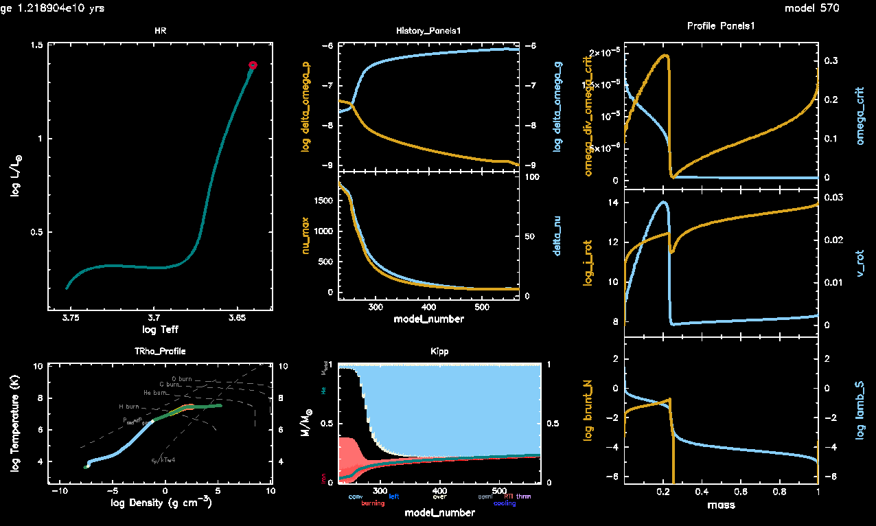
What plots you are seeing
By this point, you should be familiar with the HR diagram (top left), T-Rho Profile (bottom left), and Kippenhahn diagrams (bottom middle). The other panels will show you some important history and profile values within your model.
In the top middle panel you’ll see the JWKB estimators (on logarithmic scale) that you included into your history columns above.
In the centermost panel, you’ll see the asteroseismic values
(nu_max) and
(delta_nu). These values are explained below.
In the top 2 panels on the right hand side, you’ll see values pertaining to the rotational profile of the star, including the rotation rate
(omega_div_omega_crit), the critical rotation rate
(omega_crit), the angular momentum (log_j_rot), and the linear rotational velocity (v_rot).
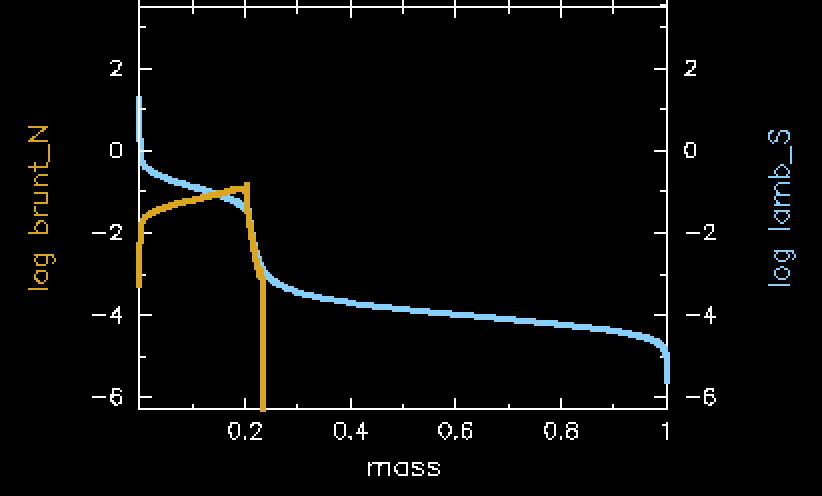
In the bottom right you’ll see the Brunt-Väisälä frequency (brunt_N) and the Lamb frequency (lamb_S). These are used to visualize a mode propagation diagram, which will be somewhat explained below, but you will also calculate your own in Lab 2.
At the end
Near the end of the red giant evolution, your pgstar output should look something like this. Notice the difference between the core and envelope rotation rates, as well as the sharp difference in the angular momentum at the core boundary.
and
In solar-like oscillators, such as the red giant we are modelling here, the oscillations excited in the star form a specific pattern, as shown below (reproduced from Garcia 2015).
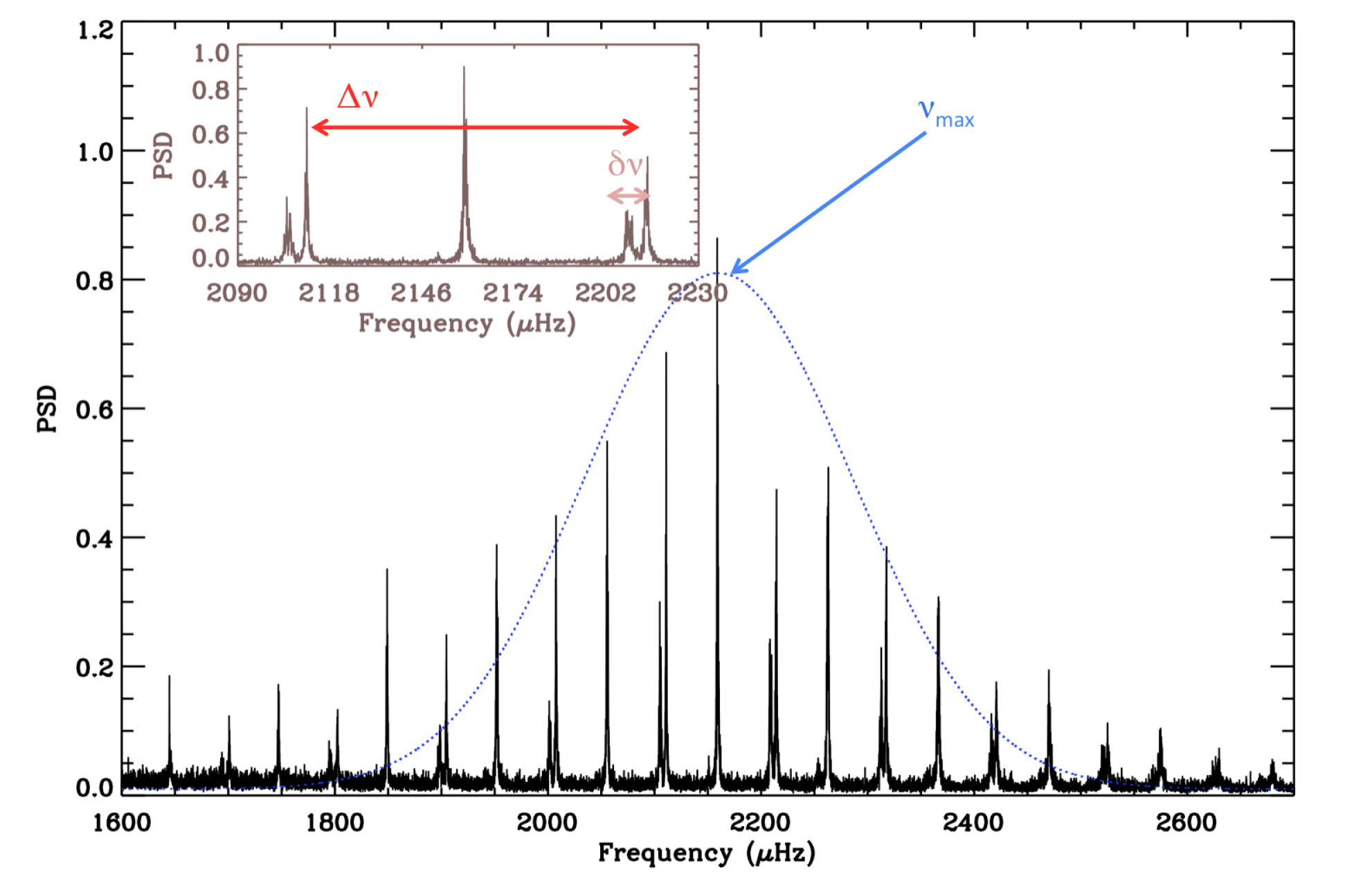
This figure also labels two important global asteroseismic parameters. First is which is roughly the central frequency of the excited oscillations, as denoted in the above figure as the mean of the blue dotted Gaussian curve. The second is or the large frequency separation, which is the frequency difference between successive radial modes (with increasing radial order ). This is denoted by the red solid arrow. This should not be confused with the small frequency separation , denoted by a small pink arrow.
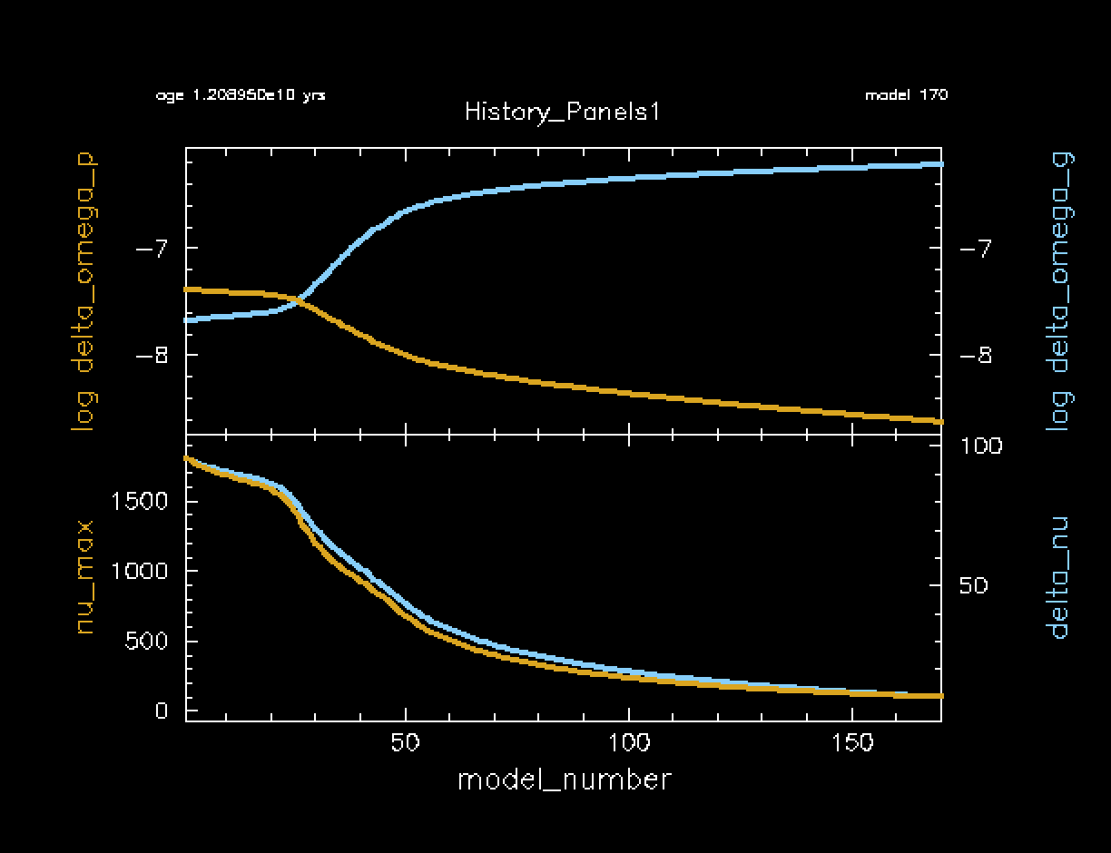
These two parameters are incredibly fundamental to solar-like asteroseismology, and can be calculated by MESA. These two parameters (nu_max and delta_nu) are plotted in the History Panels output of your rotating red giant model, as shown below. Notice how they are highly correlated to each other. In other words, they both decrease at roughly the same rate. Also notice that they both decrease as the star’s radius expands. Remember that bigger objects oscillate at lower frequencies, just like in instruments (tubas are much lower frequency than flutes, for example).
You will become more acquainted with and as you move through the labs, so don’t get discouraged if you aren’t understanding the full picture of red giant oscillations just yet!
The Mode Propagation Diagram
Stellar oscillations propagate in regions that are unstable to the stellar wave equations, which are approximated by a simple harmonic oscillator. These regions of the star are bounded by two characteristic frequencies: the Brunt-Väisälä frequency (
) and the Lamb frequency (
). These two frequencies are both functions of radius r in your stellar model.
Oscillations with frequencies smaller than both N and S in your stellar model are called g-modes and they can propagate in the g-mode cavity. Alternatively, oscillations with frequencies larger than both N and S in your stellar model are called p-modes and they propagate in the p-mode cavity.
In the pgstar output, you will see a line that corresponds to brunt_N. This indicates the Brunt-Väisälä frequency, as a function of mass coordinate within your star. Similarly, you will see a line indicating the Lamb frequency lamb_S. Specifically, this is the Lamb frequency for
, where
is the spherical degree in the spherical harmonics equations.
You will generate another representation of this mode propagation diagram in Lab 2, which will give you another opportunity to understand where the mode cavities in this star exist and how they can couple to each other.
After the run is finished - Final Task
After your run is completed, open up your history file and find the model closest to the nu_max value that you chose from the google sheet. Fill out the first five columns for your model (surface rotation rate surf_avg_omega_div_omega_crit, core rotation rate he_core_omega_div_omega_crit, delta_nu, delta_omega_p, and delta_omega_g) at the value of nu_max that you chose. Remember we’re using nu_max here as a proxy for the age of the RGB, as nu_max will decrease as the RGB star expands over time.
| 📋 TASK |
|---|
| Fill out the first five columns of the google sheet for your chosen model. |
ℹ️ HINT
nu_max is closest to your chosen value, and then scroll across to find the other values at that same time step. Feel free to use whatever method you like (i.e. python, etc) if you are familiar or if you prefer.| ❓ QUESTION |
|---|
As everyone finishes running their models and inputting their values, what do you notice about the values you’ve input into the google sheet? Compare both to the different nu_max values but also to the different initial rotation rates. |
ℹ️ ANSWER
delta_nu of each model should decrease with decreasing nu_max. 2) The surface rotation rates should decrease as nu_max decreases (age increases, radius increases). 3) The core and surface rotation rates should be different from each other.Optional Bonus: Output GYRE files at a specific numax
For Lab 2, you will be asked to calculate rotation frequencies at specific
(nu_max) values. To make this easier, you may choose to do a bonus exercise where you configure the run_star_extras.f90 file to output both profile and GYRE files when the model is at a specific
. This is not required. You can just as easily use your history file to find your calculated model closest to your desired
.
| 📋 OPTIONAL BONUS TASK |
|---|
1. Edit your src/run_star_extras.f90 file to only output profiles (and GYRE files) whenever
is at a specific, user input value. |
ℹ️ HINT 1
&controls section of inlist_1M_star and extras_finish_step in src/run_star_extras.f90.ℹ️ HINT 2
write_profiles_flag (and its corresponding value in star_info), as well as s% need_to_save_profiles_now.ℹ️ HINT 3
Counterintuitively, you will need to change your profile_interval to 1.
This is because the profile_interval will still matter even if you tell MESA to output a file in run_star_extras. So, for example if the profile closest to your
is model number 21, and your profile_interval is 5, then MESA will still skip the output of model number 21 regardless of what you tell it in run_star_extras.
ℹ️ SOLUTION
In the &controls section of inlist_1M_star:
   x_logical_ctrl(1) = .true. ! turn on for bonus task
   x_ctrl(1) = 100 ! numax
   x_ctrl(2) = 2.5 ! tolerance (change if no output)
   write_profiles_flag = .true. ! turn on for bonus task
Also in the &controls section of inlist_1M_star:
! OUTPUT PARAMS - ADJUST AS NEEDED
! NOTE YOU WILL NEED HISTORY OUTPUT AT PROFILE FOR BONUS TASK
   photo_interval = 1000
   profile_interval = 1 !!!! WAS 5 BEFORE
   history_interval = 1
   terminal_interval = 10
   write_header_frequency = 10
In extras_finish_step in src/run_star_extras.f90:
      integer function extras_finish_step(id)
        integer, intent(in) :: id
        integer :: ierr
        type (star_info), pointer :: s
        character(len=8) :: fmt, ind
        ierr = 0
        call star_ptr(id, s, ierr)
        if (ierr /= 0) return
        extras_finish_step = keep_going


	!!!!!!!!!!!!!!!!!!!!!!!!!!
        ! BONUS TASK: CAN ADD OUTPUT MANIPULATION HERE
	!!!!!!!!!!!!!!!!!!!!!!!!!!!!!!

        if (s% x_logical_ctrl(1)) then
           if ((s% nu_max < (s% x_ctrl(1) + s% x_ctrl(2))) .and. (s% nu_max > (s% x_ctrl(1) - s% x_ctrl(2)))) then
              s% write_profiles_flag = .true.
              s% need_to_save_profiles_now = .true.
              write(*,*) 'numax output now'
           else
              s% write_profiles_flag = .false.
           endif
	  endif


        if (extras_finish_step == terminate) s% termination_code = t_extras_finish_step
      end function extras_finish_step
Note that this hard-codes a tolerance of 2.5 muHz to the numax that is output. You may find that this outputs more than one profile. If you find that it outputs no models, you may need to increase this tolerance.
As always there are many methods to doing this, so your code may not look exactly like this.
Full Solutions
If you need them, a full lab 1 solution directory (including bonus task) can be downloaded here. You will still need to edit the rotation rate. The bonus task is turned off by default, unless you turn it on in the solutions. You will also need to uncomment surface rotation rate surf_avg_omega_div_omega_crit and core rotation rate he_core_omega_div_omega_crit in the history_columns.list if you use these solutions.
Troubleshooting
Input/output errors
On some systems (including HPC systems, but more generally on networked file systems), GYRE may nondeterministically fail to read or write files with i/o errors. Error messages may look like this:
HDF5-DIAG: Error detected in HDF5 (1.10.2) thread 0:
##000: ../../src/H5F.c line 445 in H5Fcreate(): unable to create file
major: File accessibilty
minor: Unable to open file
##001: ../../src/H5Fint.c line 1519 in H5F_open(): unable to lock the file
major: File accessibilty
minor: Unable to open file
##002: ../../src/H5FD.c line 1650 in H5FD_lock(): driver lock request failed
major: Virtual File Layer
minor: Can’t update object
##003: ../../src/H5FDsec2.c line 941 in H5FD_sec2_lock(): unable to lock file,
errno = 524, error message = 'Unknown error 524'
major: File accessibilty
minor: Bad file ID accessed
This is a known issue with the file locking feature as implemented in versions of the HDF5 library newer than 1.10.x (which GYRE uses for i/o operations) interacting with Linux filesystem drivers, particularly for networked drives, which may not properly implement file locking — see https://web.archive.org/web/20240508120524/https://support.nesi.org.nz/hc/en-gb/articles/360000902955-NetCDF-HDF5-file-locking. So far, Rich hasn’t come up with a fix for this. We recommend working around it by setting the following environment variable:
export HDF5_USE_FILE_LOCKING=FALSE